Equivariant neural networks  –  what, why and how ?

To motivate the merits of equivariant models in machine learning, consider the simple application of image classification. The goal is to partition the space of images into various classes:

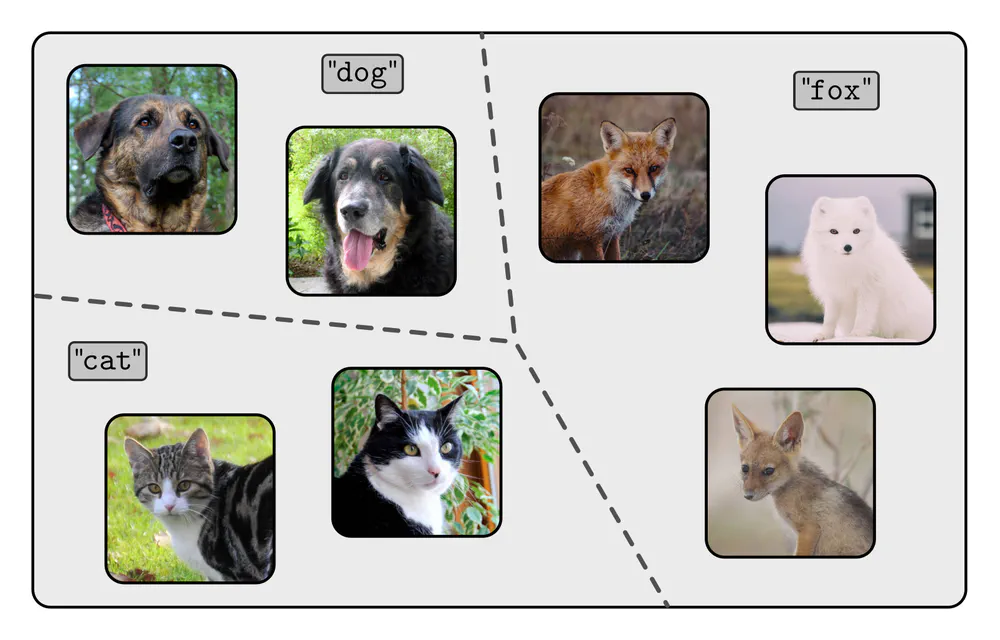
To solve this task, the classifier has to become invariant to any intra-class variabilities. For instance, there are many different appearances of fox images, and all of them should be mapped to the same class label “fox”. The intra-class variabilities are partly due to images showing truly different instances, e.g. the red and the arctic fox. In addition, “one and the same” image can occur in different appearances:

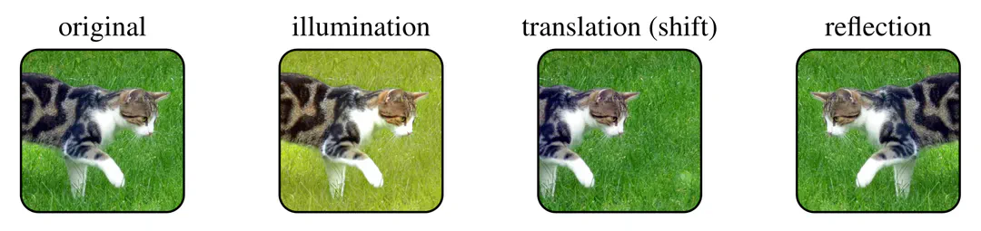
In the context of image processing or molecular modeling one would typically consider geometric transformations, like, for instance, translations, rotations, or reflections. When processing data like unordered sets the transformations of interest would instead be permutations. Mathematically, such transformations are described by symmetry groups, or, more precisely, by their group actions. An intuitive understanding of groups and their actions will be more than sufficient for this post. A more rigorous introduction to groups, actions, representations and equivariant maps in the context of deep learning can be found in Appendix B of our book.

Invariant and equivariant maps

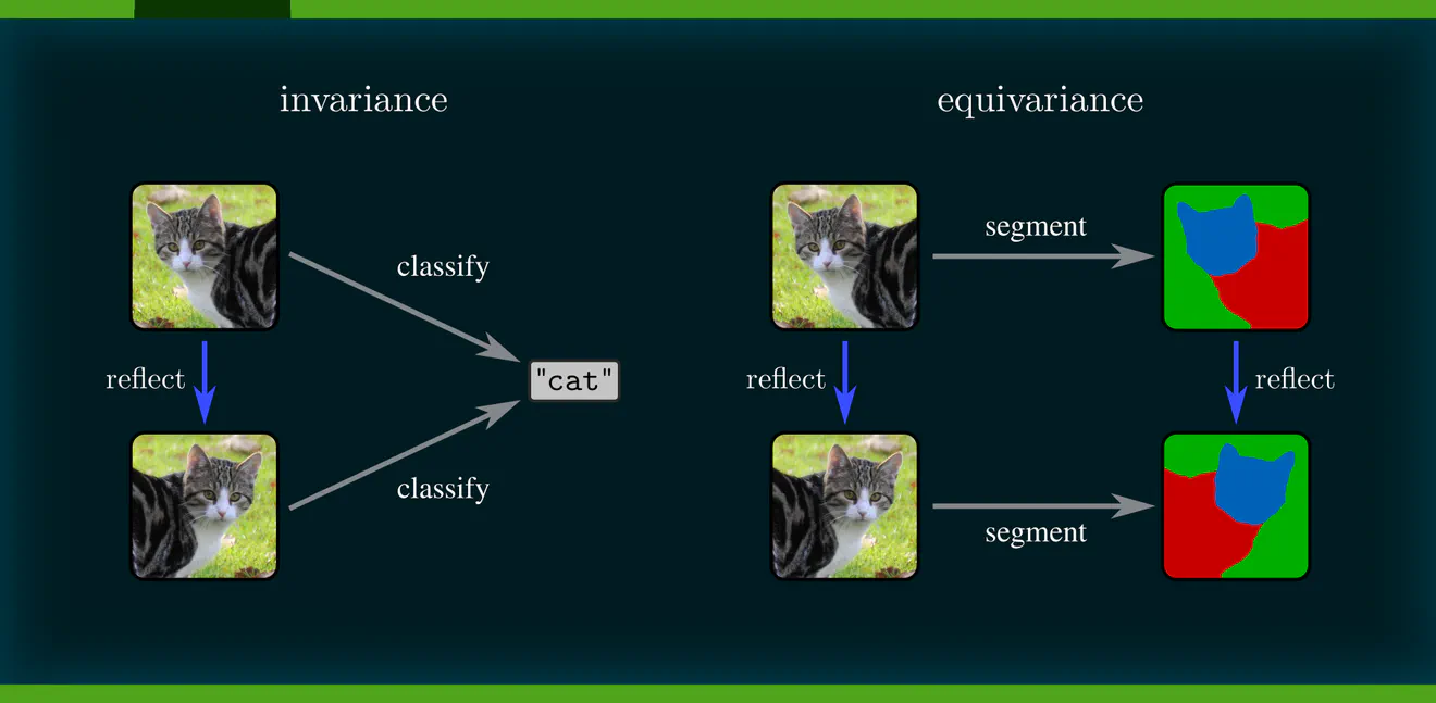
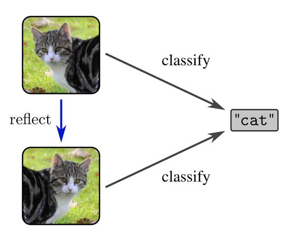
Being invariant to a geometric transformation means that the model’s prediction does not change when its input is being acted on by the transformation group. This property is visualized by the following commutative diagram, where commutativity simply means that following arrows along arbitrary paths from any start node to any end node yields the same result.

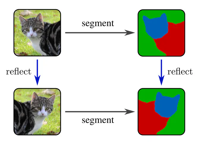
To motivate equivariance, consider an image segmentation task (pixel-wise classification) instead of image classification. The model’s output should transform here in the same way as its input. The commutativity of the diagram below captures this requirement graphically.

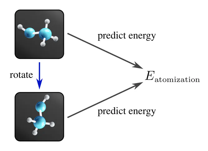
Another example of an invariant task is the prediction of a molecule’s atomization energy, which does of course not depend on the molecule’s rotation.

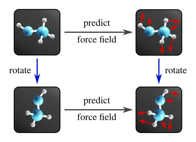
Predicting a force field is, on the other hand, an equivariant task, since the force vectors are supposed to rotate together with the molecule.

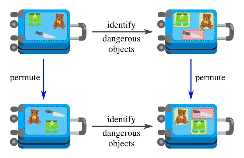
The examples above considered geometric transformations, however, similar diagrams appear in other settings as well. For instance, a classifier for detecting dangerous items in your luggage should be permutation invariant

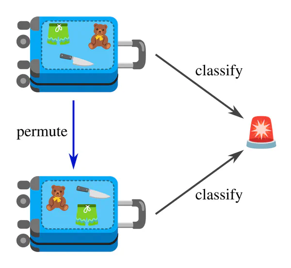
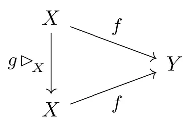
Lets try to make this a bit more formal. Firstly, invariance and equivariance are symmetry properties of functions $$f: X\to Y,$$ e.g. the classification or segmentation models above. Secondly, we need to consider some symmetry group $G$, like the reflection, rotation or permutation group. In the case of invariance, we need a group action on the domain $X$. Given any group element $g\in G$ we write $g\rhd_{\overset{}{X}} x$ for its action on any input $x\in X$. The function $f$ is then said to be $G$-invariant w.r.t. this action when it satisfies $$ f(\mkern2mu g\rhd_{\overset{}{X}} x )\ =\ f(x) \qquad \forall\ g\in G,\ \ x\in X, $$ that is, when any transformed input is mapped to the same result. This is equivalent to demanding that the following diagram commutes for any $g\in G$.

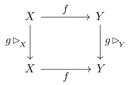
In the case of equivariance we also need a $G$-action on the codomain $Y$, which we write similarly as $g\rhd_{\overset{}{Y}} y$. Note that the domain $X$ and codomain $Y$ are in general different spaces any carry in general different group actions. $G$-equivariance of $f$ is then defined as $$ f(\mkern2mu g\rhd_{\overset{}{X}} x )\ =\ g\rhd_{\overset{}{Y}} f(x) \qquad \forall\ g\in G,\ \ x\in X, $$ which corresponds again to a commutative diagram:

How are invariant and equivariant functions related? To shed light on this question, consider a special choice of group action, the trivial action (identity map) ${g\rhd_{\overset{}{Y}} = \mathrm{id}_Y}$, which acts on $Y$ by “doing nothing”. If we use this action on the codomain of an equivariant map, the arrow form the top to bottom right collapses and we are left with an invariant function  –  invariant maps are therefore a special case of equivariant maps, such that we can talk without loss of generality about equivariant functions only.

Why should we be interested in studying the equivariance properties of machine learning models? In principle, a model would learn to be invariant or equivariant whenever this is desirable for the task it is being trained on. However, a naive model would have to learn this explicitly, that is, it would need to be shown samples in every possible transformed “pose” before it would understand their equivalence. This approach is clearly undesirable, as it leads to long training times and yields non-robust predictions.

A more sensible approach is to design the models such that they are by construction constrained to be equivariant. Instead of having to learn over and over again how to process essentially the same input, such models automatically generalize their knowledge over all considered transformations. Equivariance reduces the models’ complexity and number of parameters, which frees learning capacity, accelerates the training process, and leads to an improved prediction performance.

The probably best known equivariant network architecture are convolutional neural networks, which are translation equivariant, i.e. generalize learned patterns across space. Permutation equivariant networks, like DeepSets (Zaheer et al. 2017), are similarly guaranteed to generalize their knowledge over any reordering of input features. Using generic non-equivariant networks (i.e. multilayer perceptrons) for such tasks is practically infeasible as it would require that each input is presented in any single translated pose or any of $N!$ possible permutations, respectively.

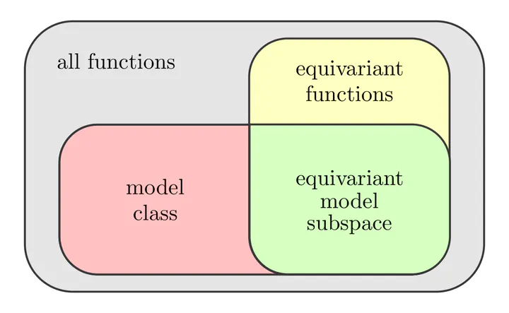
How can one guarantee the equivariance of a machine learning model? Equivariance is essentially constraining the hypothesis space of the considered model class to a lower-dimensional subspace of symmetry adapted models. The art of designing equivariant machine learning models is hence to define and parameterize these equivariant subspaces.

Before coming to equivariant neural networks further below, let’s consider the conceptually simpler example of linear regression tasks, i.e. curve fitting. In order to make an equivariant model design desirable in the first place, we need to assume certain symmetries to take advantage of. Let us therefore consider ground truth curves $f:\mathbb{R}\to\mathbb{R}$ that are either known to be symmetric or known to be antisymmetric.

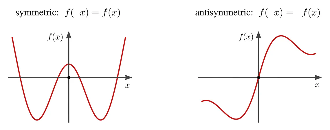
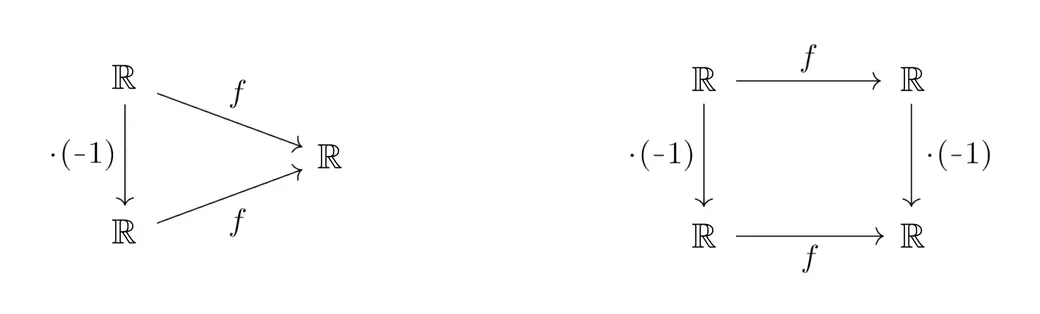
The symmetry group in this example is the reflection group, acting on the domain $\mathbb{R}$ via multiplication with $-1$, i.e. by reflecting the $x$-axis. The action on the codomain, the $y$-axis, is in the case of symmetric functions trivial, and is for antisymmetric functions again given by a multiplication with $-1$. We therefore have the following two commutative diagrams:

A naive (non-equivariant) approach to regress functions in either category would be to fit an ordinary polynomial $$y(x)\ =\ \sum_{n=0}^N w_n x^n$$ of some degree $N\in\mathbb{N}$, where the ${w_n\in\mathbb{R}}$ are ${N\mkern-2mu+\mkern-2mu1}$ trainable parameters. However, this general polynomial model would ignore our prior knowledge on the functions’ symmetry properties — they would instead have to be learned from the training data.

To take advantage of the symmetries, we can constrain the polynomial model to respect the symmetries a-priori. Doing so forces either the odd or even terms to zero, leaving us with equivariant models $$\begin{aligned} y_\textup{symm}(x)\ &= \sum_{n\ \textbf{even}}^N\ w_n x^n && (\textup{since $(-x)^n = x^n$ for even $n\in\mathbb{N}$}) \\[8pt] \textup{and}\qquad\qquad y_\textup{anti}(x)\ &= \sum_{n\ \textbf{odd}}^N\ w_n x^n && (\textup{since $(-x)^n = -(x^n)$ for odd $n\in\mathbb{N}$})\ , \end{aligned}$$ which are by design symmetric and antisymmetric, respectively. Note that these equivariant models live in subspaces with half the number of parameters in comparison to unconstrained polynomials. Furthermore, they generalize over reflections: having seen training data for $x\geq0$ only, they are automatically fitted for all $x\leq0$ as well. Twofold free lunch!

How can these principles be applied to neural networks? Viewed abstractly, a (feedforward) neural network is just a sequence $L_N\circ\dots\circ L_2\circ L_1$ of trainable layers $L_l: \mathcal{F}_{l-1}\to\mathcal{F}_l$, mapping between adjacent feature spaces:

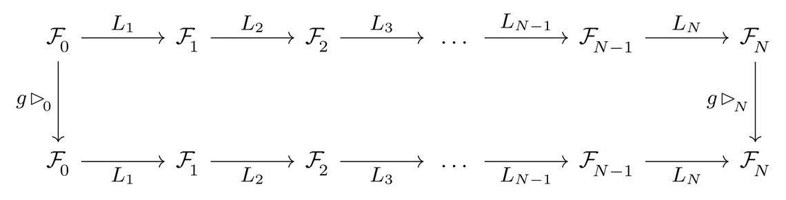
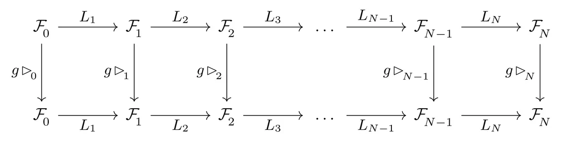
Since equivariant networks can be build in the usual modular fashion, a large part of research in equivariant deep learning is focused on developing novel equivariant layers. These layers are usually equivariant counterparts of common network operations like linear maps, bias summation, nonlinearities, message passing, attention, normalization layers, etc. The details depend hereby both on the considered symmetry group $G$ and the specific transformation laws / group actions $\rhd_{\overset{}{l}}$.

Weight sharing patterns in the neural connectivity

To build an intuition on how equivariance is incorporated into neural networks, we focus on the example of equivariant linear layers that are given by matrix multiplication. Equivariance constraints these matrices, as usual, to subspaces (so-called intertwiner spaces). They manifest themselves in weight sharing patterns in the neural connectivity that can be nicely visualized. Let’s look at some examples of groups and actions, and the implied weight sharing patterns.

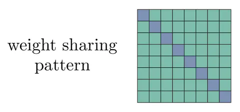
Permutations, first order actions :  A simple example are permutations $G=S_N$, acting on feature vectors $x\in\mathbb{R}^N$ by permuting their elements, that is, $[\pi\mkern-1mu\rhd\mkern-2mu x]_i := x_{\pi^{-1}(i)}$ for $i=1,\dots,N$ and any $\pi\in S_N$.

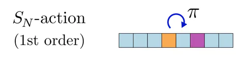
Lets assume that both of the actions $\rhd_{\overset{}{\textup{in}}}$ on the layer's input and $\rhd_{\overset{}{\textup{out}}}$ on its output are such "first order" actions. The corresponding equivariant linear maps were by Zaheer et al. (2017) shown to be given by $W = w_{\textup{id}} \mathbb{I} + w_{\textup{sum}} \mkern1mu 1\mkern1mu 1\mkern-2mu^\top$, where $\mathbb{I}$ is the identity matrix and $\mkern1mu1\mkern2mu1\mkern-2mu^\top$ is a matrix full of ones, effectively summing the elements of $x$. This constraint reduces the parameter count from $N^2$ to just $2$, as shown in the visualization for $N=8$ below (each color represents an independent parameter).

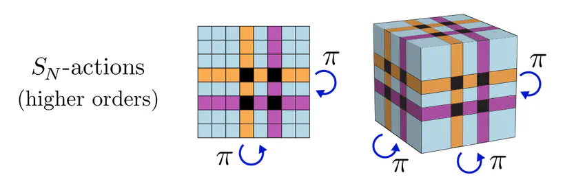
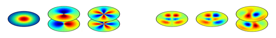
Permutations, higher order actions :  The previous result depends crucially on the specific group action that we assumed! Maron et al. (2019) allow for higher order tensor product actions of $S_N$, which transform tensors in $\mathbb{R}^{N\times\dots\times N}$ by simultaneously permuting their $k$ axes with the same group element $\pi$. The following figure shows second and third order tensors for $N=8$ as examples.

While first order actions would, for instance, model nodes of a graph, second order actions could model edges, i.e. pairs of nodes. An exemplary equivariant linear map between second order tensors for $N=5$ is shown below.

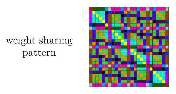
The pattern is probably not very intuitive, however, it ensures equivariance and reduces the parameter cost from 625 to 15. Even more general solutions for arbitrary $S_N$-representations (arbitrary $S_N$-actions) are discussed in (Thiede et al. 2020).

Permutation products, first order actions :  Hartford et al. (2018) investigate the setting where features correspond to $m$-tuples of elements from different sets, e.g. pairs like $(\textup{user},\textup{movie})$ ratings or triples like $(\textup{user},\textup{item},\textup{tag})$ interactions. The elements of the $m$ different sets can be permuted independently from each other. This is described by the direct product, $S_{N_1}\times\dots\times S_{N_m}$ of the individual sets' permutation groups, where $N_1,\dots,N_m$ are the sets' sizes. As data, Hartford et al. (2018) consider arrays with $m$ axes, the $j$-th of which transforms according to the first order $S_{N_j}$-action.

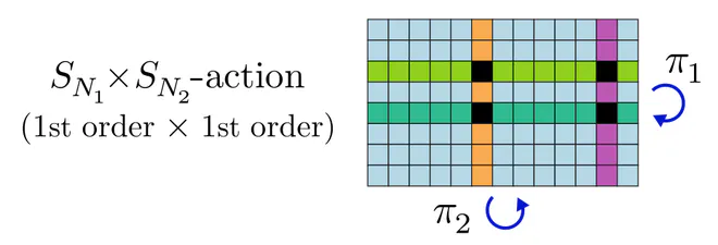
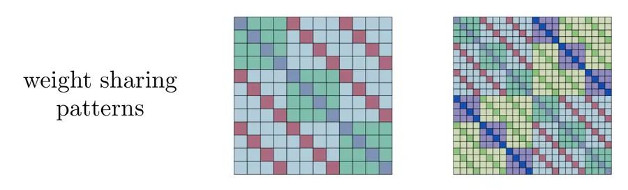
The implied weight sharing patterns turn out to be given by Kronecker products of the simple diagonal pattern of DeepSets in the first example above. This results in nested diagonal structures as shown for ${S_3\!\times\! S_4}$ and ${S_2\!\times\! S_3\!\times\! S_4}$ in the left and right plot, respectively.

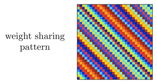
Translations, regular action :  Another important example are convolutions. To keep things simple, consider a "feature map" $x\in\mathbb{R}^N$ on the one-dimensional sampling grid ${(0,\dots,N\mkern-3mu-\mkern-3mu1)}$. Assuming cyclic boundary conditions, we can define the group $G=\mathrm{C}_N$ of cyclic translations, acting on $x$ by shifting features, i.e. $[t\rhd\mkern-1mu x]_i \,:=\, x_{(i-t) \,\mathrm{mod}\, N}$.

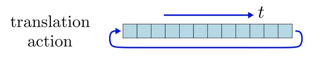
When $\rhd_{\overset{}{\textup{in}}}$ and $\rhd_{\overset{}{\textup{out}}}$ are both such shifts, the implied weight sharing pattern requires $W$ to be a circulant matrix, invariant under simultaneous shifts of its rows and columns. Note that this operation is a convolution, containing the same convolution kernel in each row shifted to another location.

Translations, invariant projection :  As a variation of the previous example we can stick with cyclic translations of the input, but seek for those linear maps that map to invariant scalar outputs. The only such mapping that is invariant under translations is weighted sum-pooling, described by a single parameter. The following visualization shows a matrix that takes a single feature map $x\in\mathbb{R}^N$ as input and contracts it with three sum-pooling maps to compute three translation invariant scalars.

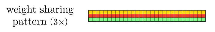
An alternative to weighted sum (or average) pooling is max-pooling, however, this would not be a linear operation!

• At initialization, register the reduced number of parameters.
• During the forward pass, 1) expand the full matrix in terms of these parameters and 2) compute the output as usual.
• Backpropagation works out of the box, with an additional step through the parameter expansion operation.

More efficient approaches might exist for simple weight sharing patterns. For example, implementing the linear layers $W = w_{\textup{id}} \mathbb{I} + w_{\textup{sum}} \mkern1mu 1\mkern1mu 1\mkern-2mu^\top$ in the first example above (DeepSets) would just require to compute and sum the weighted input and its average, instead of explicitly having to construct the matrix $W$.

General solutions:  The examples above all assume certain permutation actions of finite groups, for which Ravanbakhsh et al. (2017) presented a full characterization of equivariant linear maps. A representation theoretic formulation allows to derive even more general solutions, where $G$ need not be finite. This solution relies on decompositions of the representations into irreducible representations, for which the solutions are implied by Schur’s lemma. More details can be found in Appendix E of our book. An alternative, numerical approach relying on Lie algebra representations is described in (Finzi et al., 2021).

• The feature spaces of equivariant networks are equipped with some choice of group actions that the layers need to respect. Mathematically, they are not just vector spaces, but group representation spaces.
• Equivariant networks can be constructed in a modular fashion, i.e. by chaining individually equivariant layers. The group actions on the previous layers' output feature space needs to agree with those on the following layers' inputs.
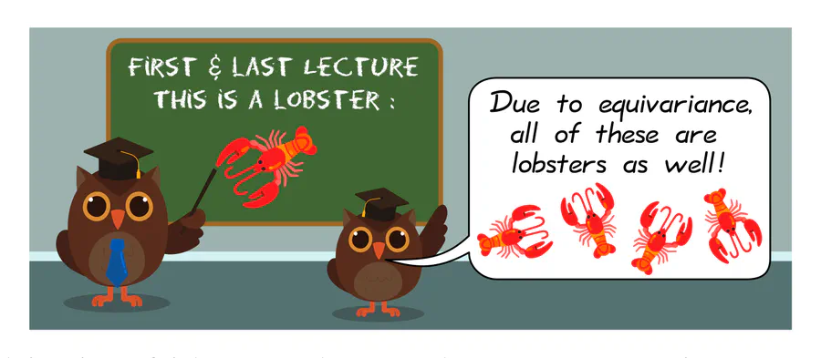
• Equivariance ensures the consistency of predictions under symmetry transformations: an equivariant model generalizes anything it learns to all transformed inputs.
• Equivariant layers live in subspaces with a reduced parameter count. The operations in these subspaces exhibit characteristic weight sharing patterns.
• As a consequence of the last two points, equivariant models are more data efficient, less prone to overfitting, and converge faster in comparison to non-equivariant models.

If you want to learn more about the group representation theory of convolutional neural networks (CNNs), you can read on in the next post of this series. It explains feature maps as representation spaces and derives CNN layers as equivariant maps between them. Translation equivariance results thereby in the characteristic spatial weight sharing patterns of CNNs, which require that one and the same operation (e.g. kernel) needs to be applied at each location.

The post thereafter studies generalized equivariant CNNs which commute with extended groups of symmetries, including, e.g., rotations or reflections. As we will see, the extended equivariance enforces additional weight sharing patterns (or symmetries) in the convolution kernels themselves: