Convolutional networks  &  translation equivariance

Convolutional neural networks (CNNs) are the standard network architecture for spatially structured signals, like images, audio, videos, or tensor fields in the physical sciences. They differ from plain, fully connected networks in two respects:

1. They usually have a local neural connectivity.
2. They share synapse weights (e.g. a convolution kernel) between different spatial locations.

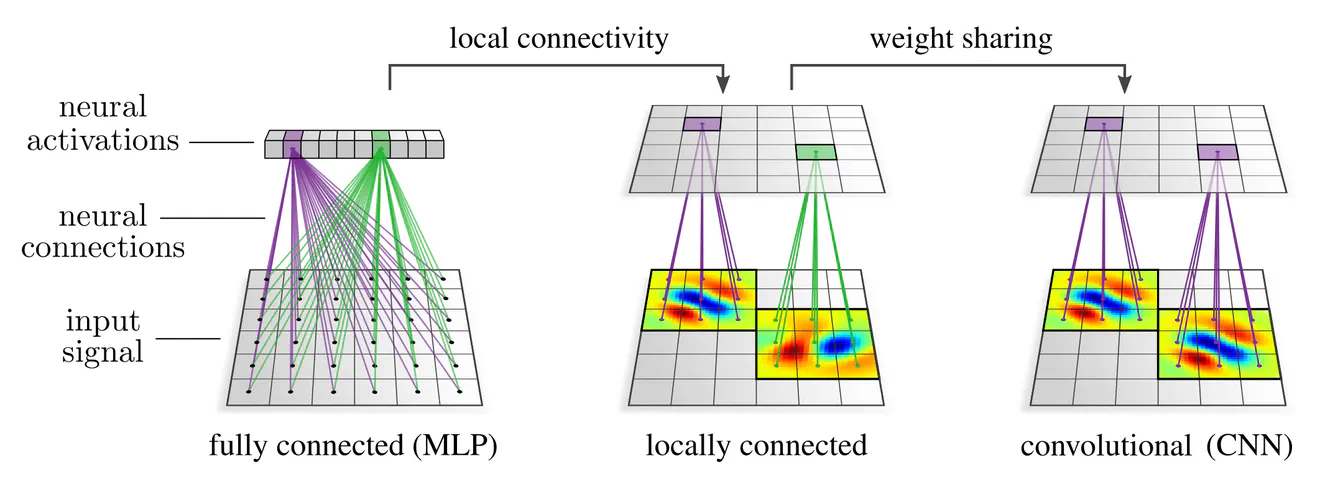
CNNs owe their name to so-called convolution operations, which are exactly those linear maps that share weights. Intuitively, convolutions can be thought of as sliding a template pattern – the convolution kernel – across space, matching it at each single position with the signal to produce a response field. However, the weight sharing requirement applies not only to linear maps, but to any type of operation employed in convolutional networks. It also enforces, for instance, that one and the same bias vector or the same nonlinearity is to be used at every spatial position.

Both the local connectivity and weight sharing reduce the number of model parameters (visualized by the number and color of the synapse weights in the graphics above), which makes CNNs less hungry for training data in comparison to fully connected networks. The local connectivity implies in addition that each neuron is associated with a specific spatial location (the center of its receptive field), such that they are naturally arranged in “feature maps”.

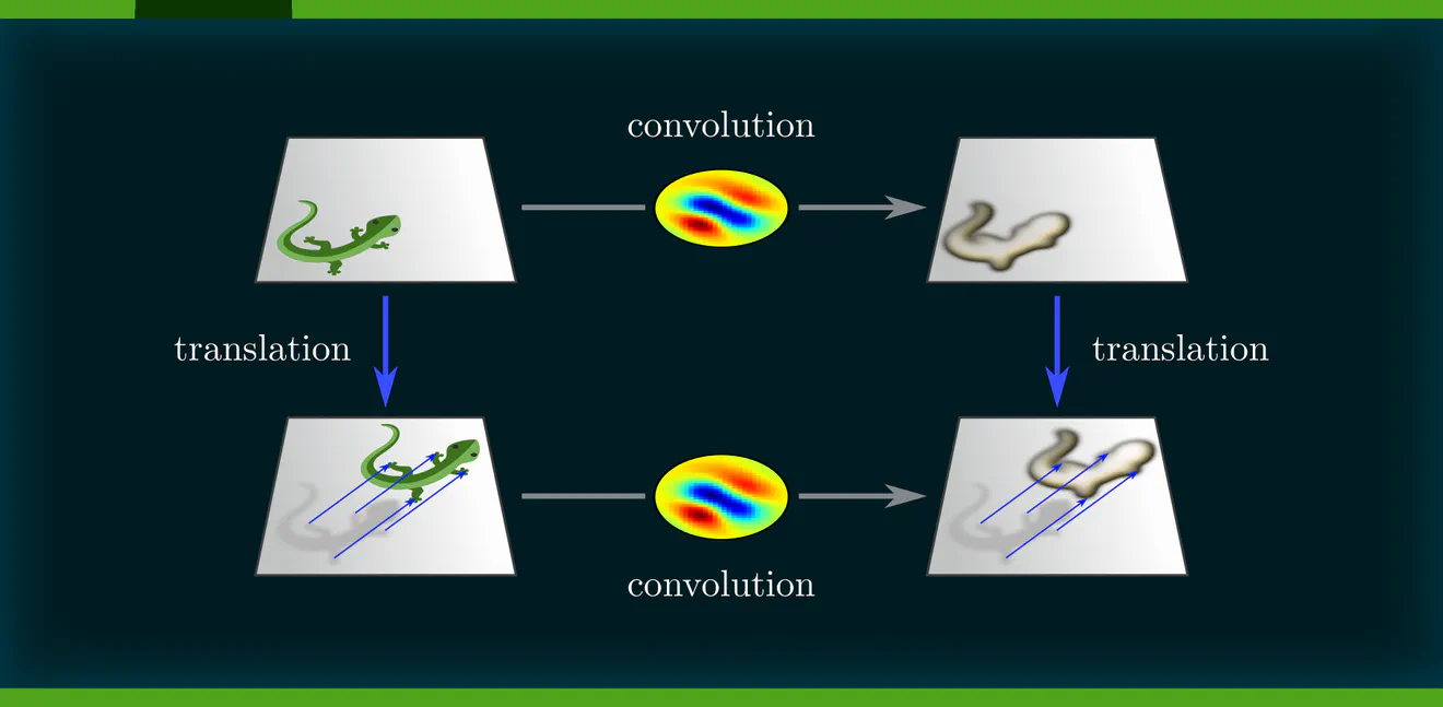
More important for us is, however, that the spatial weight sharing implies the translation equivariance of convolutional networks: $$\textup{spatial weight sharing} \quad\Longrightarrow\quad \textup{translation equivariance}$$ To see intuitively that this is indeed the case, note that any translation of a network’s input shifts patterns to other neurons’ receptive fields. Given that the neural connectivity is shared, these neurons are guaranteed to evoke the same responses as those at the previous location  –  CNN layers commute therefore with translations!

Instead of defining convolutional networks as sharing weights, and subsequently observing that they happen to be equivariant, one can reverse the implication arrow and derive weight sharing by demanding their equivariance: $$\textup{spatial weight sharing} \quad\Longleftarrow\quad \textup{translation equivariance}$$ We define conventional CNNs therefore equivalently as those neural networks that are translation equivariant.

Feature maps as translation group representations

To substantiate this statement we need to formalize the feature spaces of CNNs as group representation spaces  –  feature maps need to be equipped with translation group actions w.r.t. which network layers should commute.

In discretized implementations, feature maps are commonly sampled on a regular grid and numerically represented by an array of shape $(X_1,\dots,X_d\,,C)$, where $X_1,\dots,X_d$ are $d$ spatial dimensions and $C$ is a number of channels. For instance, an RGB image has $C=3$ channels and $d=2$ spatial dimensions, with $X_1$ and $X_2$ being its height and width in pixels.

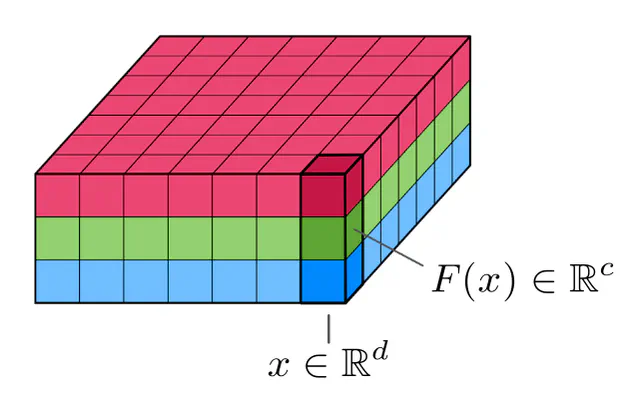
In the continuous settings, feature maps are modeled as functions $$ F:\, \mathbb{R}^d \to \mathbb{R}^c, $$ which assign feature vectors $F(x)\in\mathbb{R}^c$ to each spatial location $x\in\mathbb{R}^d$. Assuming the usual summation and scalar multiplication of functions, the spaces of such feature maps become (feature) vector spaces.

To turn these feature spaces into translation group representations we define translation group actions on them. We are interested in those specific actions $\rhd$ of the translation group $(\mathbb{R}^d,+)$ which transform feature maps by shifting them around. They are for any translation $t\in(\mathbb{R}^d,+)$ given by $$ \big[\mkern1.5mu t\rhd F \big](x) \ :=\ F(x-t) \,, $$ which means that the value of the translated feature map ${t\mkern-1mu\rhd\mkern-3mu F}$ at any ${x\in\mathbb{R}^d}$ is taken from the original feature map $F$ at ${x-t}$.

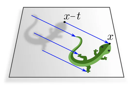
The vector space of feature maps with this action is known as regular representation of the translation group. A more precise definition of the spaces of feature maps is given here.

CNN layers as translation equivariant maps

1. map input feature maps $F: \mathbb{R}^d \to \mathbb{R}^{c_\textup{in}}$ to output feature maps $\mathcal{L}(F): \mathbb{R}^d \to \mathbb{R}^{c_\textup{out}}$, and
2. are translation equivariant, that is, commute with any translations $t\in(\mathbb{R}^d,+)$ : $$ \mathcal{L}(t\rhd F)\ =\ t\rhd \mathcal{L}(F) \,. $$

As explained in the previous post, equivariant layers are commonly derived from standard, non-equivariant operations, like general linear maps, bias summation, nonlinearities, and so on. Independent from the specific type of operation, translation equivariance of a layer requires the translation invariance of its neural connectivity, i.e. spatial weight sharing. The following paragraphs give specific examples.

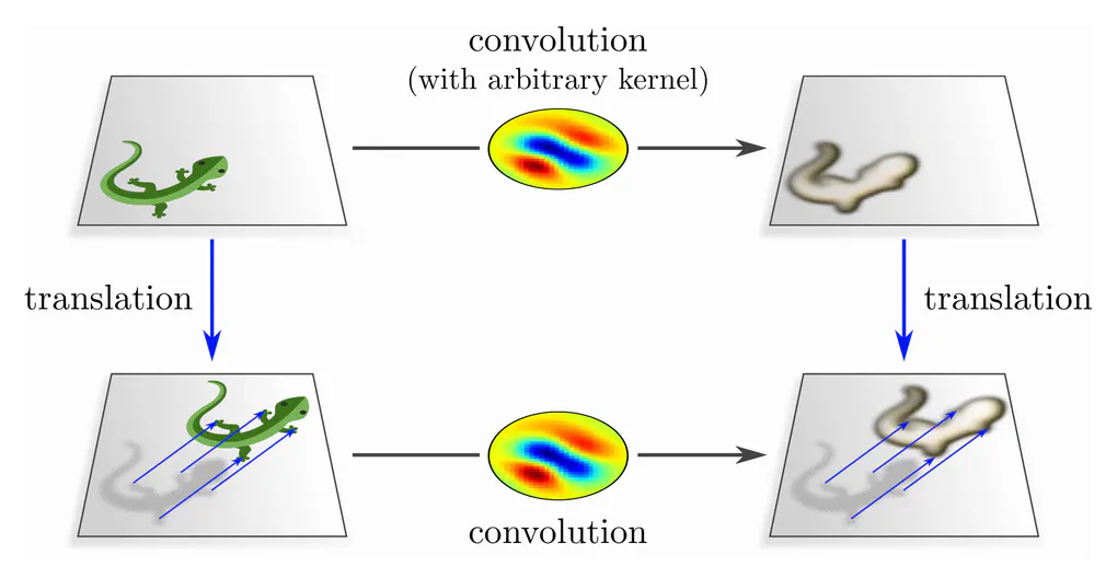
Linear layers:  The most basic type of neural network operations are linear layers. Our central theorem on conventional CNNs asserts:

Translation equivariant linear functions between feature maps are necessarily convolutions ${K\!\ast\mkern-2mu F}$.

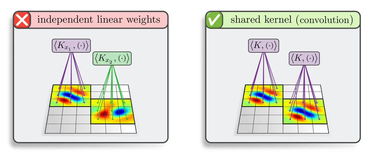
Given that feature maps are vector-valued with $c_\textup{in}$ input channels and $c_\textup{out}$ output channels, the convolution kernel $K$ needs to be ${c_\textup{out}\!\times\! c_\textup{in}}$ matrix-valued. When being sampled on a discrete grid with a kernel size of ${S_1\!\times\!\dots\!\times\! S_d}$ pixels, it is encoded as an array of shape $(S_1,\dots,S_d\,,C_\textup{out},C_\textup{in})$. This corresponds in continuous space to a matrix-valued function $K: \mathbb{R}^d \to \mathbb{R}^{c_\textup{out}\times c_\textup{in}}$.

The local connectivity of CNNs, corresponding to a kernel with compact support, does not follow from equivariance, but is an independent design choice.

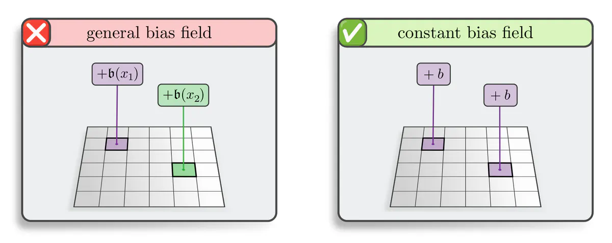
Bias summation:  Another standard operation is bias summation. In full generality, one could sum different bias vectors $\mathfrak{b}(x)\in\mathbb{R}^{c_\textup{in}}$ to feature vectors $F(x)\in\mathbb{R}^{c_\textup{in}}$ at different locations $x\in\mathbb{R}^d$, that is, one could sum an unconstrained bias field $\mathfrak{b}: \mathbb{R}^d \to \mathbb{R}^{c_\textup{in}}$ to feature maps $F: \mathbb{R}^d \to \mathbb{R}^{c_\textup{in}}$. However, we prove:

Translation equivariance requires bias fields to be spatially constant,
that is, $\mathfrak{b}(x) = b$ for some $b\in\mathbb{R}^{c_\textup{in}}$ and any $x\in\mathbb{R}^d$.

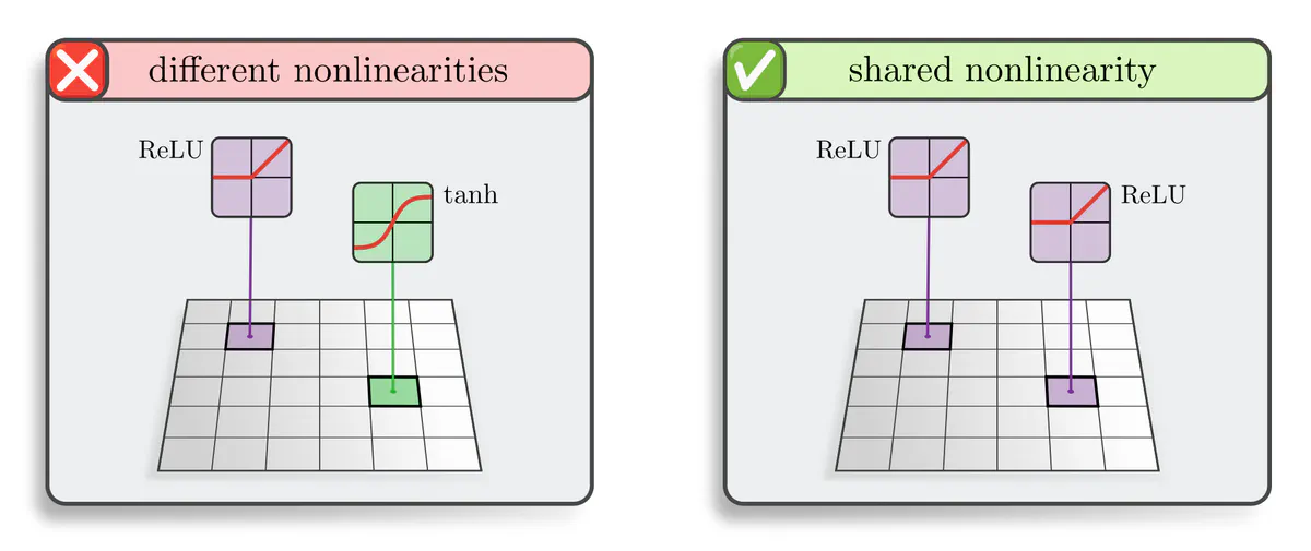
Nonlinearities:  Activation functions in CNNs are usually applied pointwise, i.e. individually to each feature vector. One could in principle apply different nonlinearities at different locations, e.g. a $\mathrm{ReLU}$ at one point and $\tanh$ somewhere else. However, equivariance requires – once again – weight sharing:

The same nonlinearity needs to be applied at each point when translation equivariance is demanded.

Pooling:  Yet another example are local pooling operations, which compute the output feature vector at any location $x$ by aggregating a patch of input features within a local pooling region around $x$. It is probably little surprising by now that:

Translation equivariant pooling operations need to apply the same pooling region at each location.

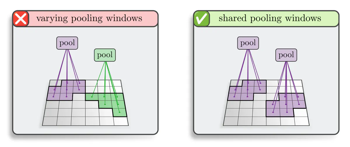
We prove this statement in the continuous setting. It holds in the discrete setting as well when a "stride" of 1 pixel is used. Larger strides correspond to subsampling operations, which reduce the networks' equivariance to a subgroup of strided translations. An interesting alternative are the fully equivariant subsampling operations by Xu et al. (2021), which rely on the idea to predict the subsampling grids themselves in an equivariant (comoving) manner.

There is one more translation group representation of interest in conventional CNNs, namely the trivial representation, which models translation invariant features. It appears in CNNs after applying global pooling operations, which are translation invariant functions that send feature maps (regular representations) to invariant features (trivial representations).

A limitation of the representation theoretic description of CNNs is that it is only able to explain global translations of feature fields as a whole. It is intuitively easy to see that CNNs with locally supported kernels are equivariant under more general independent translations of local patterns in the kernels’ field of view.

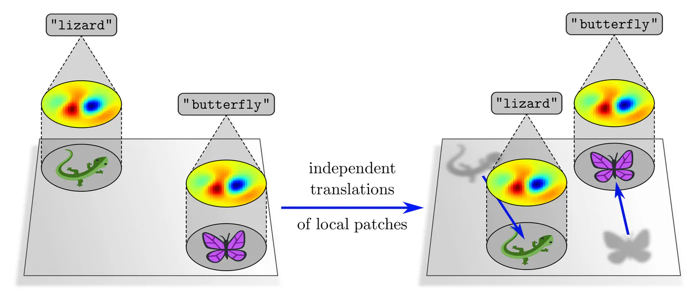
This phenomenon is of great practical relevance since it covers global translations as a special case, but additionally explains transformations like the movement of a foreground object relative to a background scene, or the generalization of CNNs over low-level features like corners and edges, which reappear at arbitrary locations in images. Our gauge theoretic formalism, covered in the last post of this series, investigates such and more general local transformations in greater detail.

The key insight in this post is that there is a mutual implication $$ \begin{array}{c} \textup{translation equivariant} \\ \textup{network layers} \end{array} \quad\iff\quad \begin{array}{c} \textup{translation invariant neural connectivity} \\ \textup{(spatial weight sharing)} \end{array} $$ which allows to derive the convolutional network design purely from symmetry principles. Feature maps are thereby identified as regular translation group representations, and CNN layers are defined as equivariant maps between these representation spaces.

The next post investigates analogous definitions of generalized equivariant CNNs by means of requiring their layers’ equivariance under extended groups of geometric transformations, including e.g. rotations or reflections. As there are additional symmetries involved, these models are subject to generalized weight sharing constraints ("$G$-steerability"), which we will analyze in detail.