Equivariant CNNs & G-steerable kernels
An introduction to equivariant & coordinate independent CNNs – Part 3
This post is the third in a series on equivariant deep learning and coordinate independent CNNs.
- Part 1: Equivariant neural networks – what, why and how ?
- Part 2: Convolutional networks & translation equivariance
- Part 3: Equivariant CNNs & G-steerable kernels
- Part 4: Data gauging, co variance and equi variance
- Part 5: Coordinate independent CNNs on Riemannian manifolds
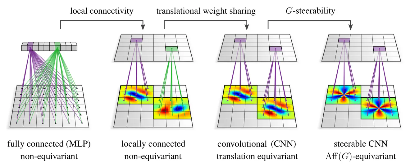
The previous post investigated the mutual implication “weight sharing $\Leftrightarrow\mkern-2mu$ translation equivariance” that is underlying conventional CNNs on Euclidean spaces. In this post we will define generalized equivariant CNNs by leveraging analogous implications for extended groups of geometric transformations, including e.g. rotations or reflections of feature vector fields. As we will see, such equivariant CNNs rely generally on convolutions with “steerable convolution kernels”, which are kernels that obey additional symmetry constraints.
This post discusses:
- Affine symmetry groups, with respect to which we demand CNNs to be equivariant.
- The weight sharing patterns implied by affine group equivariance.
- $G$-steerable kernels – first the abstract idea, then explicit examples.
- Empirical results which highlight the advantages of steerable CNNs.
- The generality of our mathematical formulation and its relation to alternative approaches.
The content of this post is more thoroughly covered in our book on Equivariant and Coordinate Independent CNNs, specifically in chapters four (affine equivariant CNNs), five (steerable kernels), and six (experiments).
If you are interested in applying equivariant CNNs, make sure to check out our PyTorch extension escnn!
The first question we have to ask ourselves when building equivariant models is which symmetry group we are interested in. Let’s consider some typical learning tasks and their appropriate levels of symmetry.
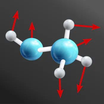
- The first visualization shows a molecule, embedded in $\mathbb{R}^3$, for which one might want to predict binding energies or a force field. As the underlying physics is invariant under translations, rotations, and reflections, any neural network for such applications should commute with these actions. For instance, a rotated molecule should result in a rotated force field.
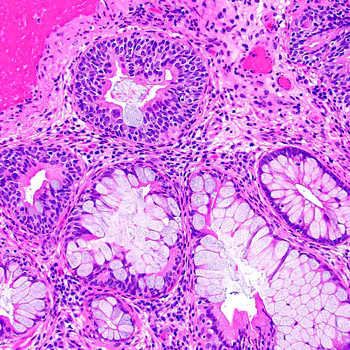
- A common task in biomedical imaging is to scan histological sections for malignant tissue. Such images possess usually no preferred choice of origin or orientation. Neural networks for processing such data should therefore again be equivariant under translations, rotations and reflections, however, in this case in $d=2$ dimensions.
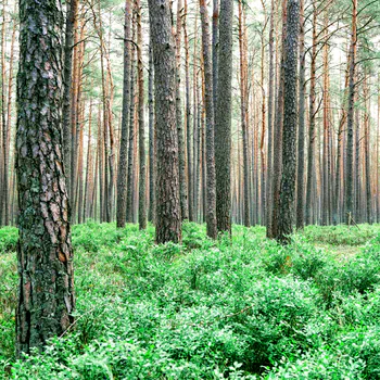
- Gravity imposes a preferred direction in the third example, breaking the rotational symmetry. Translations and horizontal reflections are still relevant. Furthermore, objects at different distances appear at a different scale, suggesting the utility of dilation equivariance.
How are these transformations described mathematically? Translations take a distinguished role as they act on Euclidean space $\mathbb{R}^d$ via summation. The other transformations, i.e. rotations, reflections and dilations, act via matrix multiplication. Multiplications with matrices include furthermore any other linear transformations, for instance, shearing.
Translations are modeled by the translation groups $(\mathbb{R}^d,+)$. The other transformations are, in general, described by general linear groups $\mathrm{GL}(d)$, i.e. the groups of all invertible ${d\mkern-3mu\times\mkern-4mu d}$–matrices. In practice, we are not necessarily interested in making our model equivariant w.r.t. all such linear transformations. Instead, we consider matrix subgroups $$G\mkern2mu\leq\mkern2mu\mathrm{GL}(d),$$ which gives us the flexibly to select subsets of transformations. Examples would be pure rotations $G=\mathrm{SO}(d)$, rotations and reflections $G=\mathrm{O}(d)$, or volume-preserving transformations $G=\mathrm{SL}(d)$.
Taken together, translations and $G$-transformations form so-called affine groups $$ \mathrm{Aff}(G)\ :=\ (\mathbb{R}^d,+) \rtimes G. $$
Don’t worry if you are wondering about the
semidirect product symbol
The key insight of the previous post was that there is a mutual implication $$\textup{translational weight sharing} \quad\iff\quad \textup{translation group equivariance},\mkern10mu$$ which was leveraged to derive conventional CNN layers by demanding their equivariance. We define generalized $\mathrm{Aff}(G)$-equivariant CNN layers by means of analogous relations $$\textup{affine weight sharing} \quad\iff\quad \textup{affine group equivariance}$$ for affine groups. We therefore need to understand and implement the weight sharing patterns that $\mathrm{Aff}(G)$-equivariance imposes on the neural connectivity.
To analyze these patterns, recall that affine groups consist of
- translations $(\mathbb{R}^d,+)$, and
- additional $G$-transformations.
- translational weight sharing – just as for conventional CNNs – and
- additional weight sharing over $G$-actions, formalized by so-called "$G$-steerability " constraints.
Of course, we still need to understand what exactly it means for the neural connectivity to be $G$-steerable. The following two sections clarify this question by discussing the general idea of steerable kernels and going through examples for specific groups and group actions.
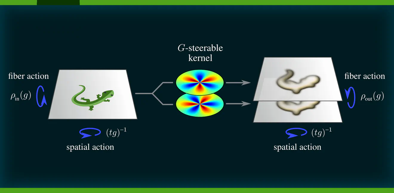
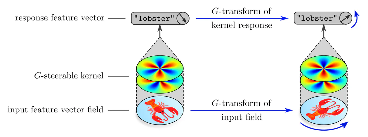
Apart from their symmetry constraints, steerable kernels are just convolution kernels as found in conventional CNNs. Recall from the previous post that such kernels are by definition ${c_\textup{out}\mkern-3mu\times\mkern-3mu c_\textup{in}}$ matrix-valued when they are supposed to map between feature fields with $c_\textup{in}$ and $c_\textup{out}$ channels, respectively. We visualize such matrix-valued kernels in the following as matrices of kernels:
In a nutshell, the
The specific transformation law according to which the response feature vector should transform is thereby specified by some choice of
$G$-representation $\rho$
,
which is a hyperparameter of the model.
Intuitively, such feature vectors can be thought of as simultaneously encoding
the $G$-invariant content, e.g.
Applied at one single location, a kernel produces a single response feature vector, as shown above. Convolutions apply a kernel at every point of space, and result therefore in a whole feature vector field. Since convolutions are translation equivariant, and steerable kernels are $G$-equivariant, any convolution with a steerable kernel is jointly translation and $G$-equivariant – they are hence $\operatorname{Aff}(G)$-equivariant, as desired.

The main challenge in constructing $\operatorname{Aff}(G)$-equivariant CNNs is to solve for and to parameterize the subspaces of $G$-steerable convolution kernels. Each subspace of steerable kernels is thereby characterized by the specific choice of matrix group $G$ and the group representations $\rho_{\textup{in}}$ and $\rho_{\textup{out}}$ according to which their input and output feature vectors are supposed to transform.
To get a more concrete understanding of the functioning of steerable kernels, let’s consider some simple examples where $G$ are rotations or reflections in $d=2$ dimensions.
Reflection steerable kernels
The simplest non-trivial example is the one where $G$ is the reflection group, such that $\operatorname{Aff}(G)$ consists of translations and reflections.
Assume the convolution input to be a scalar field, modeling, for instance, a grayscale image. Let the convolution kernel be symmetric, i.e. invariant under reflections. When being applied to a reflected input such a kernel is guaranteed to produce exactly the same responses as for the original input, however, now located at spatially reflected positions. As the output field transforms in this example just like the input field, it is of scalar type as well.
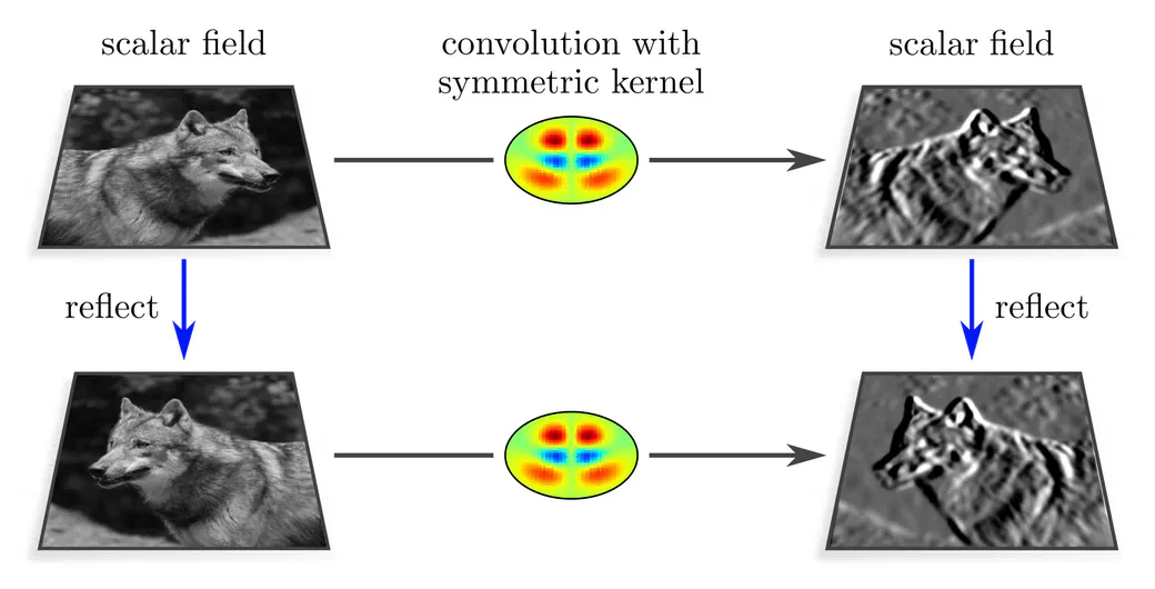
Note that general, non-symmetric kernels would not satisfy this equivariance diagram. Their two response fields on the right-hand side would rather be mutually unrelated.
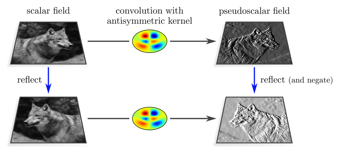
Next, let us consider antisymmetric kernels, which negate under reflections. Due to this property, the response field to a spatially reflected scalar input field will not only appear spatially reflected, but will additionally change its sign. This transformation behavior is a valid reflection group action, corresponding to so-called pseudoscalar fields.
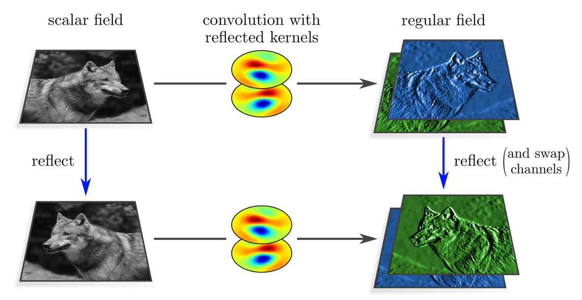
As a third example, we assume a kernel with two output channels, the second of which is a reflected copy of the first one. When reflecting the input field, its orientation relative to the second (first) kernel channel agrees with that of the original input and the first (second) kernel channel. A reflection of the input field results therefore in a response field which is spatially reflected and whose two channels are swapped. Feature fields that transform in this manner are called regular feature fields.
Let’s have a look at how the response fields transform. In all three cases, they are reflected spatially. The fields’ feature values at each individual location remain in the case of scalar fields invariant, are in the case of pseudoscalar fields negated, and experience a channel swapping in the case of regular fields. These transformations correspond to
$G$-representations $\rho$ that act on the channel dimension (i.e. on feature vectors).
Specifically, scalars transform according to the trivial representation, pseudoscalars according to the sign-flip representation, and regular feature vectors according to the regular representation of the reflection group. Further $G$-representations would correspond to more general field types.| group element | scalar field trivial representation | pseudoscalar field sign-flip representation | regular field regular representation |
|---|---|---|---|
| identity | $\begin{pmatrix}1\end{pmatrix}$ | $\begin{pmatrix}1\end{pmatrix}$ | $\begin{pmatrix}1&0\\0&1\end{pmatrix}$ |
| reflection $\vphantom{\rule[-25pt]{0pt}{0pt}}$ | $\begin{pmatrix}1\end{pmatrix}
\vphantom{\Bigg|\rule[-14pt]{0pt}{0pt}}$ (leaves channel invariant) | $\begin{pmatrix}-1\end{pmatrix}
\vphantom{\Bigg|\rule[-14pt]{0pt}{0pt}}$ (negates channel) | $\begin{pmatrix}0&1\\1&0\end{pmatrix}
\vphantom{\Bigg|\rule[-14pt]{0pt}{0pt}}$ (swaps channels) |
In the above analysis, we assumed a specific input field type and reflection steerable kernels to be given, from which the output field type followed: $$ \mkern36mu \begin{array}{c} \textup{input field type $\rho_{\textup{in}}$} \\[2pt] \textup{$G$-steerable kernel} \end{array} \quad\Longrightarrow\quad \textup{output field type }\rho_{\textup{out}} \mkern40.5mu $$ In practice, we are, conversely, fixing desired input and output field types, and derive the corresponding subspaces of steerable kernels that map equivariantly between them: $$ \begin{array}{c} \textup{input field type $\rho_{\textup{in}}$} \\[2pt] \textup{output field type $\rho_{\textup{out}}$} \end{array} \quad\Longrightarrow\quad \textup{$G$-steerable kernels} \mkern36mu $$ Specifically for scalar inputs and for outputs described by trivial, sign-flip, or regular representations, these subspaces contain exactly the symmetric, antisymmetric, and “reflected-copy” kernels above. The table below visualizes further solutions for other combinations of input and output field types. Try to assert that the kernels’ $G$-symmetries are indeed respecting the assumed transformation laws!
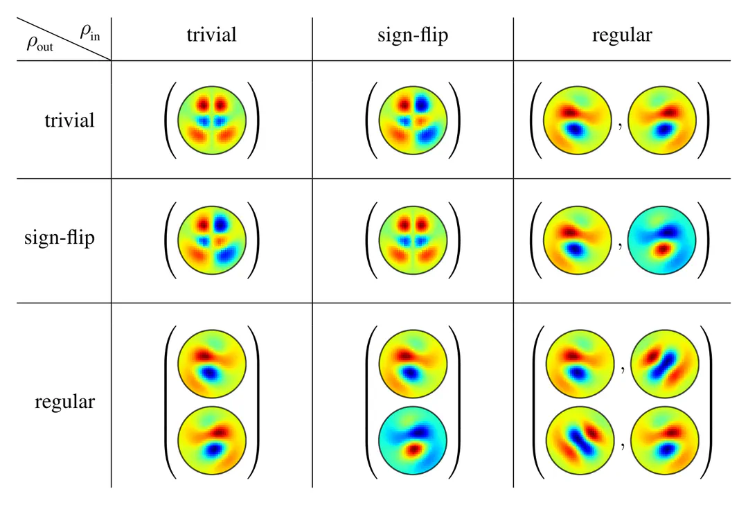
A mathematical derivation of these kernels can be found here. Note that their reflectional symmetries imply that they are two times more parameter efficient in comparison to conventional kernels. If you are interested in how such steerable kernels can be implemented in practice, check out this repository.
Rotation steerable kernels
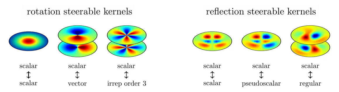
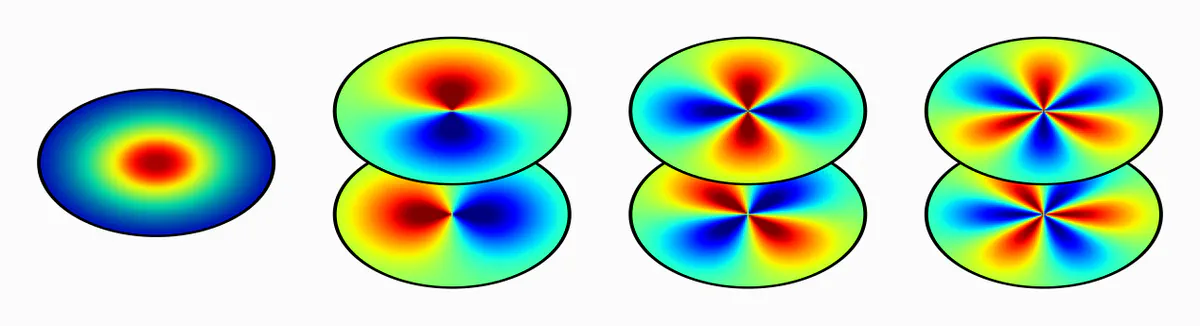
As a second example, we consider the rotation group $G=\operatorname{SO}(2)$ in two dimensions. Just as reflection-steerability imposes reflection symmetry constraints on the kernels, rotation-steerability imposes certain rotational symmetries. Independent from the specific constraint, which depends again on the field types $\rho_{\textup{in}}$ and $\rho_{\textup{out}}$, it is clear that rotation steerability constrains the kernels' angular parts, but does not affect their radial parts.
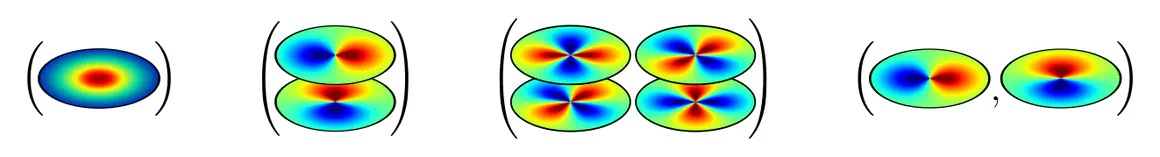
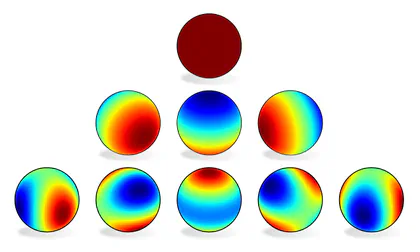
The visualization below shows exemplary kernels mapping between scalar and vector fields, which have, respectively, ${c\mkern-2mu=\mkern-2mu1}$ and ${c\mkern-2mu=\mkern-2mu2}$ channels on $\mathbb{R}^2$.
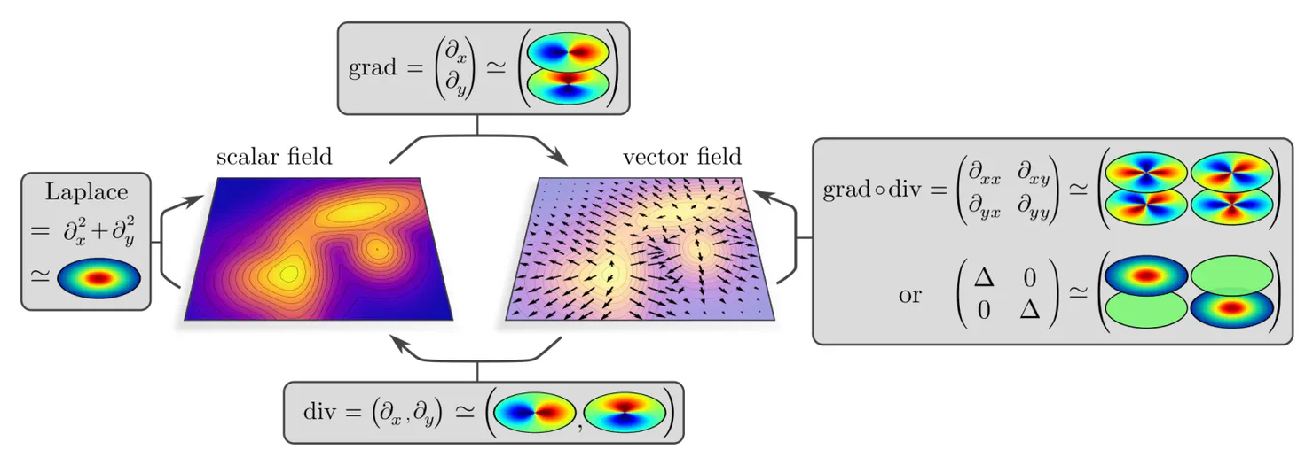
These kernels can be viewed as spatially extended counterparts of well-known partial differential operators (PDOs), like the Laplacian (scalar$\mkern2mu\to\mkern0mu$scalar ), gradient (scalar$\mkern2mu\to\mkern0mu$vector ), divergence (vector$\mkern2mu\to\mkern0mu$scalar ), or gradient of the divergence and a channel-wise Laplacian (vector$\mkern2mu\to\mkern0mu$vector ). This resemblance to common PDOs appearing in the natural sciences is no coincidence – due to the rotational symmetries of the laws of nature, these operators need to be equivariant, i.e. steerable in the very same sense as our convolution kernels! Such steerable partial differential operators are characterized in (Jenner and Weiler 2021).
More general solutions than those visualized above exist: for instance, $\mathrm{SO}(2)$-steerability would allow for angular phase-shifts (any rotation of the kernels), and the unconstrained radial parts would get optimized during the training process. For more expressive steerable kernel spaces, which allow for higher angular frequencies and the mixing of multiple different frequencies, one needs to consider more complex field types, e.g. general tensor fields or regular representations. A full overview of the complete solution spaces of $\operatorname{SO}(2)$ and $\operatorname{O}(2)$-steerable kernels can be found here.
Is all the complicated representation theory worth the effort? All empirical evidence in our experiments and in the literature shows that equivariant CNNs bear a significant potential to improve the model performance on any machine learning tasks that involve the processing of spatial signals.
For instance, the following plot shows that the convergence rates and the final validation losses of CNNs improve with an increasing level of equivariance. The cyclic groups $G=\mathrm{C}_N$ in this experiment are discrete approximations of continuous rotations in $\mathrm{SO}(2)$, containing $N$ rotations by multiples of $\frac{2\pi}{N}$.
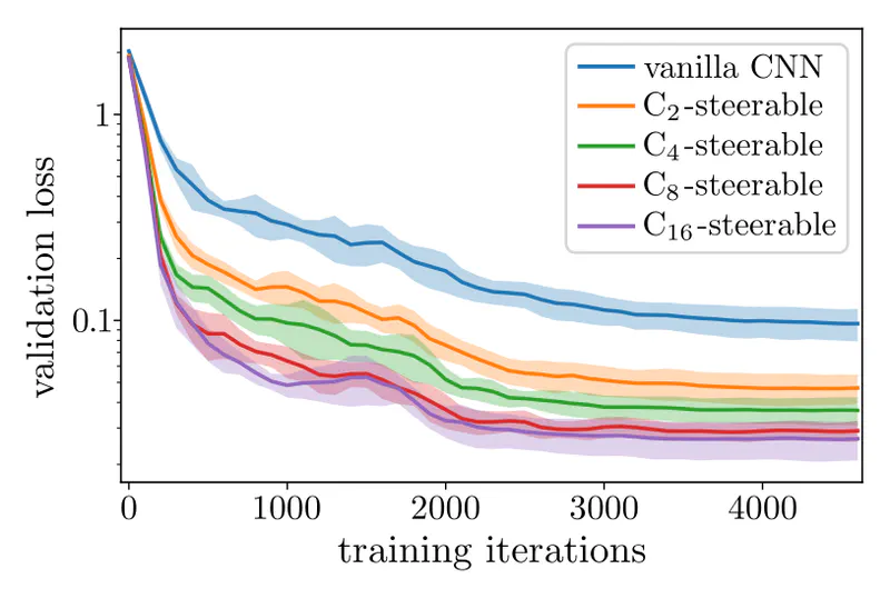
The faster convergence of equivariant CNNs relates to their enhanced data efficiency :
each training sample is automatically generalized to any $G$-transformed pose,
such that less samples need to be presented before the network learns a given task.
A particularly impressive result by
Winkels and Cohen (2019)
shows that steerable CNNs can achieve the same performance like a baseline CNN
despite being trained on
The following table shows test errors of a conventional CNN baseline in comparison to rotation and reflection steerable CNNs on three different image classification datasets. Since equivariant CNNs are more parameter efficient we ran two models: the first one keeps the number of channels fixed and has less parameters, while the second one increases the number of channels such that the number of parameters is held constant. Without any hyperparameter tuning, i.e. just by plugging in steerable kernels etc., both models achieve significantly better test errors than their baseline.
| model | CIFAR-10 test error (%) | CIFAR-100 test error (%) | STL-10 test error (%) |
|---|---|---|---|
| CNN baseline | $ 2.6 \pm 0.1 $ | $17.1 \pm 0.3 $ | $12.74\pm 0.23$ |
| E(2)-CNN (same number of channels) | $ 2.39\pm 0.11$ | $15.55\pm 0.13$ | $10.57\pm 0.70$ |
| E(2)-CNN (same number of params) | $ 2.05\pm 0.03$ | $14.30\pm 0.09$ | $ 9.80\pm 0.40$ |
We got similar improvements for steerable CNNs in three-dimensional space that are trained to classify randomly $\mathrm{SO}(3)$-rotated objects from the ModelNet10 dataset. The different models in the table assume different matrix groups $G\leq\mathrm{SO}(G)$; see (Cesa et al., 2022) for more details.
| model | rotated ModelNet10 test error (%) |
|---|---|
| CNN baseline | $17.5 \pm 1.4 $ |
| SO(2)-CNN (z-axis) | $13.1 \pm 1.9 $ |
| Octa-CNN | $10.3 \pm 0.6 $ |
| Ico-CNN | $10.0 \pm 0.6 $ |
| SO(3)-CNN | $10.5 \pm 1.0 $ |
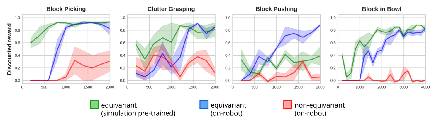
Further impressive results were presented by Wang et al. (2022), who used our library escnn for training equivariant policies for robotic arms that are supposed to manipulate physical objects given a visual input. As the curves in the plots below show, the policies that are based on steerable CNNs are able to learn the task, while the non-equivariant baseline does not even converge.
More experiments on steerable CNNs can be found in the sixth Chapter of our book.
Why should we care specifically about steerable CNNs, given that there exist many alternative formulations of equivariant CNNs in the literature? The reason is that
Steerable CNNs are a general theoretical framework for equivariant convolutions
which unify most alternative approaches in a coherent representation theoretic language.
While other formulations are usually focussing on very specific choices of groups and group actions (i.e. field types $\rho$), steerable CNNs allow for arbitrary groups and any actions that result in convolutions . Steerable CNNs clarify how the different approaches relate to each other and show that their convolution operations are ultimately all relying on one or the other type of $G$-steerable kernels.
To substantiate these claims, we give some examples of popular equivariant CNN models and discuss how they are explained from the viewpoint of steerable CNNs.
Harmonic Networks: Worrall et al. (2017) proposed to build $\mathrm{SE}(2)$-equivariant networks based on circular harmonic kernels. These are exactly those $\mathrm{SO}(2)$-steerable kernels corresponding to field types $\rho$ that are irreducible representations of $\mathrm{SO}(2)$.
Tensor Field Networks: $\mathrm{E}(3)$-equivariant networks are commonly based on convolutions with spherical harmonics, followed by a Clebsch-Gordan decomposition operation; see e.g. (Thomas et al., 2018). These operations correspond to convolutions with $\mathrm{O}(3)$-steerable kernels, where the field types $\rho$ are the irreducible representations of $\mathrm{O}(3)$.
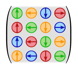
Group convolutions: The probably most popular equivariant network design are group equivariant convolutional networks (Cohen and Welling, 2016). Their mathematical formulation may seem quite different from that of steerable CNNs, however, we prove that they are just another special case, corresponding to regular representations $\rho$. The kernels' weight sharing pattern (steerability) for 90-degree rotations in $G=\mathrm{C}_4$ is shown on the right.
Quotient space convolutions: Related to group convolutions are the convolutions on quotient spaces by Kondor and Trivedi (2018) and Bekkers (2020). Once again, they are just a special case of steerable convolutions, this time assuming quotient representations as field types.
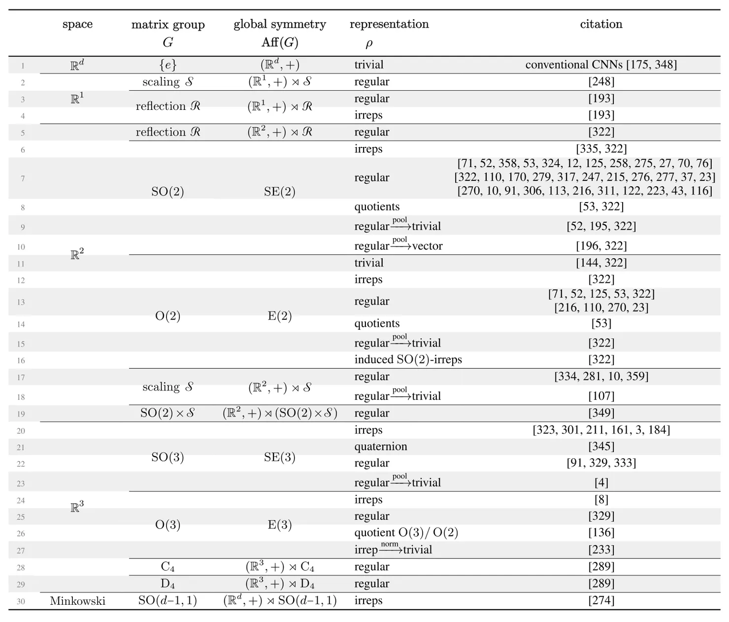
This list goes on and on. The table below shows many more models from the literature that we identified as instantiations of steerable CNNs for different spaces, groups and $G$-representations.
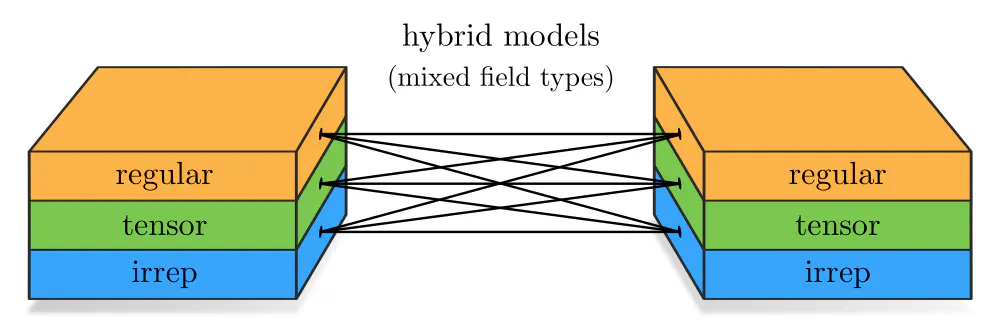
Note that steerable CNNs do not only allow to reconstruct all of these architectures in isolation, but explain additionally how to build hybrid models which operate on different field types simultaneously. For example, a feature space can at the same time contain regular feature fields, any tensor fields, and fields corresponding to irreducible representations (irreps). Our library escnn will automatically construct the appropriate steerable kernels for mapping between any pairs of field types in use.
Another important difference of our approach is that we derive the steerability constraints from first principles. In contrast, alternative approaches usually come up with steerable kernels heuristically, i.e. introduce them as some construction which happens to be equivariant. Our steerable kernels are provably complete, meaning that we are guaranteed that they model the most general equivariant linear maps for given field types.
The main takeaways of this post are:
- Steerable CNNs on Euclidean spaces are equivariant under actions of affine groups $\mathrm{Aff}(G)$, where $G\leq\mathrm{GL}(d)$ can be any (sub)group of ${d\mkern-3mu\times\mkern-4mu d}$–matrices.
- Feature fields are equipped with $\mathrm{Aff}(G)$-actions.
The specific actions depend on their field type,
which is a choice of
$G$-rep resentation $\rho$, determining the transformation law of individual feature vectors. - The translation symmetries in affine groups result in spatial weight sharing, just as in conventional CNNs. The $G$-transformations imply additional $G$-steerability constraints.
- Steerable kernels map feature fields of type $\rho_\textup{in}$ to fields of type $\rho_\textup{out}$ (e.g. scalar$\mkern2mu\to\mkern0mu$vector). The specific $G$-symmetries imposed by steerability constraints depend on these input and output field types.
- In contrast to other approaches, ours allows to derive steerable kernels and to prove the completeness of steerable kernel spaces. It applies furthermore to arbitrary groups and group actions, and unifies the model zoo of equivariant CNNs in a unified representation theoretic language.
- Empirically, generalized equivariant CNNs show major advantages in comparison to merely translation equivariant CNN baselines.
Further reading :
As you might have noticed, I avoided a technical definition of feature fields, resorting to examples and geometric intuition. Check out Section 4.2 of our book if you are interested in a more formal (yet quite intuitive) definition of feature fields as elements of induced representation spaces.
I also skipped over a mathematical definition of the $G$-steerability constraints, which is discussed in Chapter 5 of our book. As proven in (Lang and Weiler, 2020), steerable kernels are mathematically equivalent to quantum representation operators (e.g. spherical tensor operators), and are therefore described by a generalization of the famous Wigner-Eckart theorem. $G$-steerability constraints between field types can be viewed as an analog to transition rules between quantum states – only certain operators (kernels) may map between given input and output states (fields).
To prevent the post from getting even longer, I didn't include steerable biases and nonlinearities. If you are interested in them, you will find a short introduction and examples in the bonus section below (click on the title to expand the content).
Outlook :
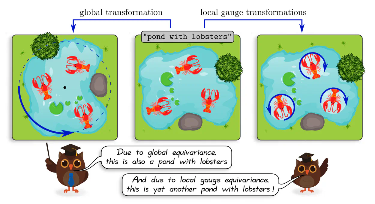
Equivariant CNNs are classically designed with global transformations in mind: the model should, for instance, commute with rotations or reflections of feature fields as a whole. As discussed above, this generally requires $G$-steerability, i.e. the property of kernels to be equivariant under $G$-transformations of their input. If the kernel has a compact support, which is standard practice for compact $G$, it is intuitively plausible that independent $G$-valued "gauge transformations" of the kernels' fields of view at different locations lead to independent $G$-transformations of their responses.
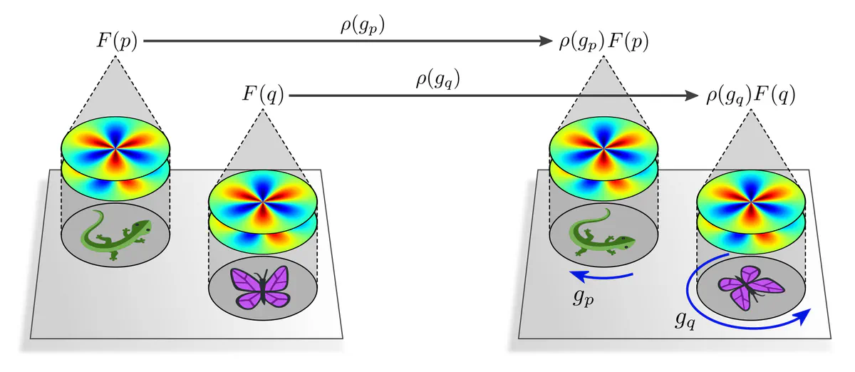
Steerable CNNs will therefore not only generalize their knowledge over global transformations in $\mathrm{Aff}(G)$, but also over any $G$-transformations of local patterns!
To formalize this intuition mathematically, one needs to reformulate CNNs in a gauge theoretic language. The next post of this series gives a first introduction to gauges and gauge transformations in deep learning, applying to arbitrary data modalities and to neural networks in general. A gauge field theory of convolutional networks is covered in the post after that.
Bonus section (click to expand):
The steerability constraints do not only apply to convolution kernels, but to any (spatially shared) operation that is used in an equivariant network, in particular to biases and nonlinearities. Since biases and nonlinearities are applied pointwise, i.e. to individual feature vectors, their steerability constraints are significantly simpler than those of spatially extended kernels, which are applied to a whole field of feature vectors in their field of view. In a nutshell, one finds that
$G$-steerable bias summation and nonlinearities need to commute with
the
$G$-representations
$\rho_{\textup{in}}$ and $\rho_{\textup{out}}$
that act on their input and output feature vectors.
Steerable bias summation
In the
previous post
we discussed that the summation of a bias vector field is only then translation equivariant when this field is translation invariant, i.e. determined by a single shared bias vector:
$$\mkern5mu
\textup{translation invariant bias field}
\quad\iff\quad
\textup{translation equivariant bias summation},
$$
We prove an analogous
theorem
which asserts that the bias field is required to $\mathrm{Aff}(G)$-invariant
when demanding that its summation to a feature fields is an $\mathrm{Aff}(G)$-equivariant operation:
$$
\mathrm{Aff}(G)\textup{-invariant bias field}
\quad\iff\quad
\mathrm{Aff}(G)\textup{-equivariant bias summation}
$$
This implies again spatial weight sharing, however,
the shared bias vector $b$ is further constrained to be
Let’s clarify this by looking at some examples:
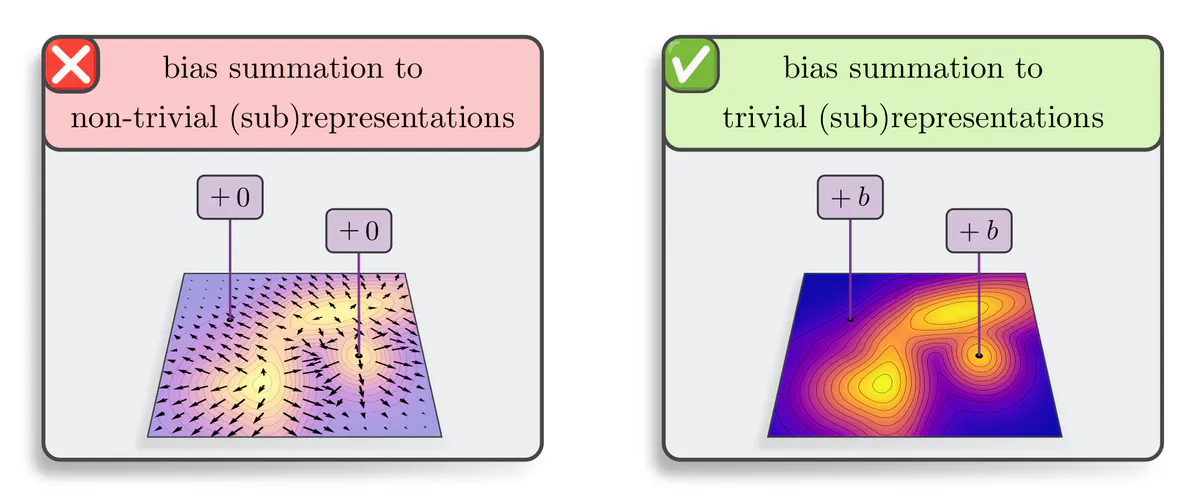
- Scalar fields are, by definition, described by trivial representations $\rho(g)=1$. Due to the $G$-invariance of scalars, one may sum any scalar bias $b\in\mathbb{R}$ to them. This holds for any choice of $G.$
- Pseudoscalar fields transform according to the sign-flip representation. As it contains no trivial subrepresentation, bias summation is forbidden. Intuitively, summing a bias to an original or a negated field is only then equivalent when the bias is equal zero.
- The tangent vector fields for $G=\mathrm{SO}(2)$ are similarly disallowing bias summation: the only bias tangent vector $b\in\mathbb{R}^2$ that commutes with rotations of feature tangent vectors is the zero-vector.
- The feature vectors of regular feature fields do (for any $G$) contain exactly one trivial subrepresentation, to which one may sum a bias. For the reflection group example, this corresponds to summing $b=(\beta,\beta)$ with $\beta\in\mathbb{R}$ to the two channels. As the same parameter $\beta$ is summed to each channel, this operation commutes with the channel swapping action of the regular representation. Click here if you would like to see how this relates to an irrep decomposition of the regular representation.
Steerable nonlinearities
A similar
theorem
holds for nonlinearities:
they need to be shared over spatial positions and need to be
- For scalar fields we have one channel $c_{\textup{in}}=1$ and the trivial representation $\rho_{\textup{in}}(g)=1$. One may therefore use any nonlinearity and a trivial output representation $\rho_{\textup{out}}$, for which the constraint becomes trivial.
- If $\rho_{\textup{in}}$ is the sign-flip representation, modeling pseudoscalar fields, one can no longer apply any nonlinearity. For instance, using a $\mathrm{ReLU}$ would suppress negative values and keep positive ones, however, after reflecting and negating the field, the negative and positive values would switch their role! Any valid nonlinearity may only act on the field's norm, which stays invariant under negation. One could, for example, use antisymmetric activation functions like $\tanh$.
- A similar argument holds for the tangent vector fields for $G=\mathrm{SO}(2)$: A rotation of a vector $(0,1)^\top$ by $\pi/2$ gives $(-1,0)$. This rotation does obviously not commute with $\mathrm{ReLU}$-nonlinearities. One may again use any nonlinearity that acts on the vector's norms – this holds more generally for any unitary representations.
- Regular representations are permutation representations, which commute generally with any nonlinearity that is applied channel-wise. For instance, for the reflection group example it does not matter whether $\mathrm{ReLU}$ activations are applied to the two channels before or after they are swapped.
Finding the most suitable steerable nonlinearities for a given field type is pretty much still an open research question. We ran extensive benchmark experiments to compare some of the most popular choices.
Maurice Weiler
Deep Learning Researcher
I’m a researcher working on geometric and equivariant deep learning.
Image references
- Molecule image adapted from macrovector on Freepik.
- Histology image from Maria Tretiakova on PathologyOutlines.com.
- Forest photo from Stefan Haderlein on Pexels.
- Animations of affine transformations adapted from Felix Liu's blog post on "Understanding Transformations in Computer Vision".
- Lobsters adapted under the Apache license 2.0 by courtesy of Google.
- Lizards and butterflies adapted under the Creative Commons Attribution 4.0 International license by courtesy of Twitter.
- Wolf photo adapted from Nicky Pe on Pexels.
- Owl teacher adapted from Freepik
- On-robot learning reward curves adapted from Wang et al. (2022)