Data gauging,  co variance  and  equi variance

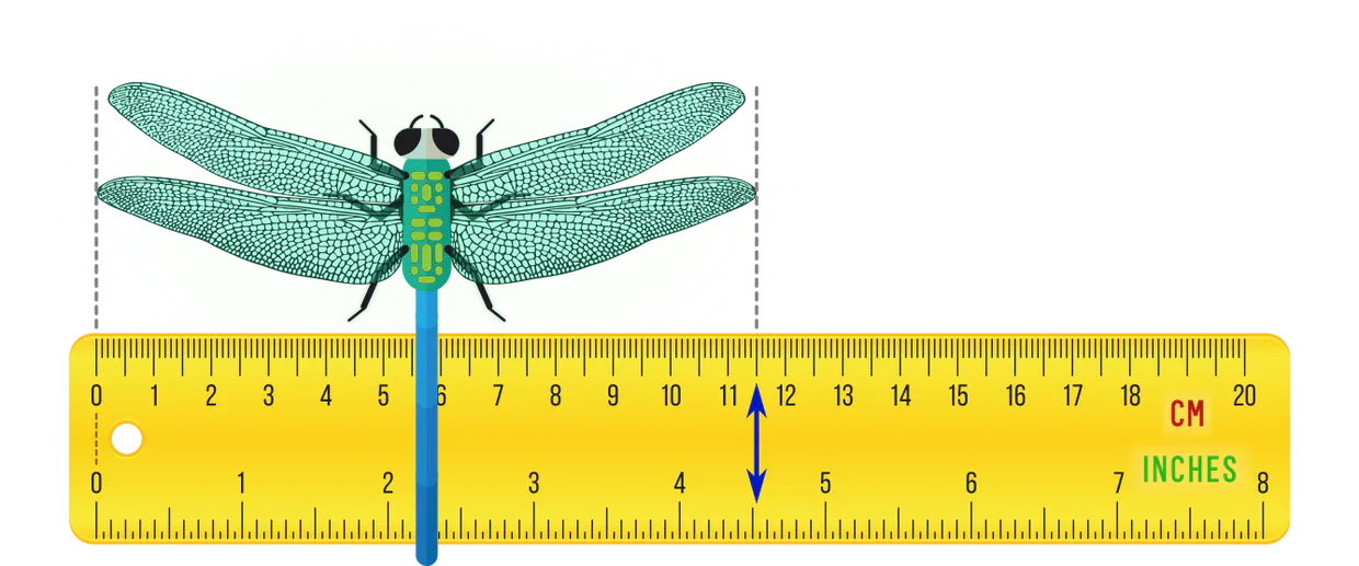
Gauge theories regulate redundancies in the mathematical description of data or other mathematical objects. A simple example from everyday life is that one may use different yet equivalent units of measurement, e.g. centimeters vs. inches for distances, or kilograms vs. pounds to measure weight. The specific choice of units (the gauge) is ultimately arbitrary since we can always convert between them (perform gauge transformations).

Neural networks crunch numbers  –  it is therefore necessary to numerically quantify data like physical lengths or masses by picking some gauge. A consistent gauge theoretic description simply ensures that the predictions of a network or theory remain independent from the particular choice of gauge.

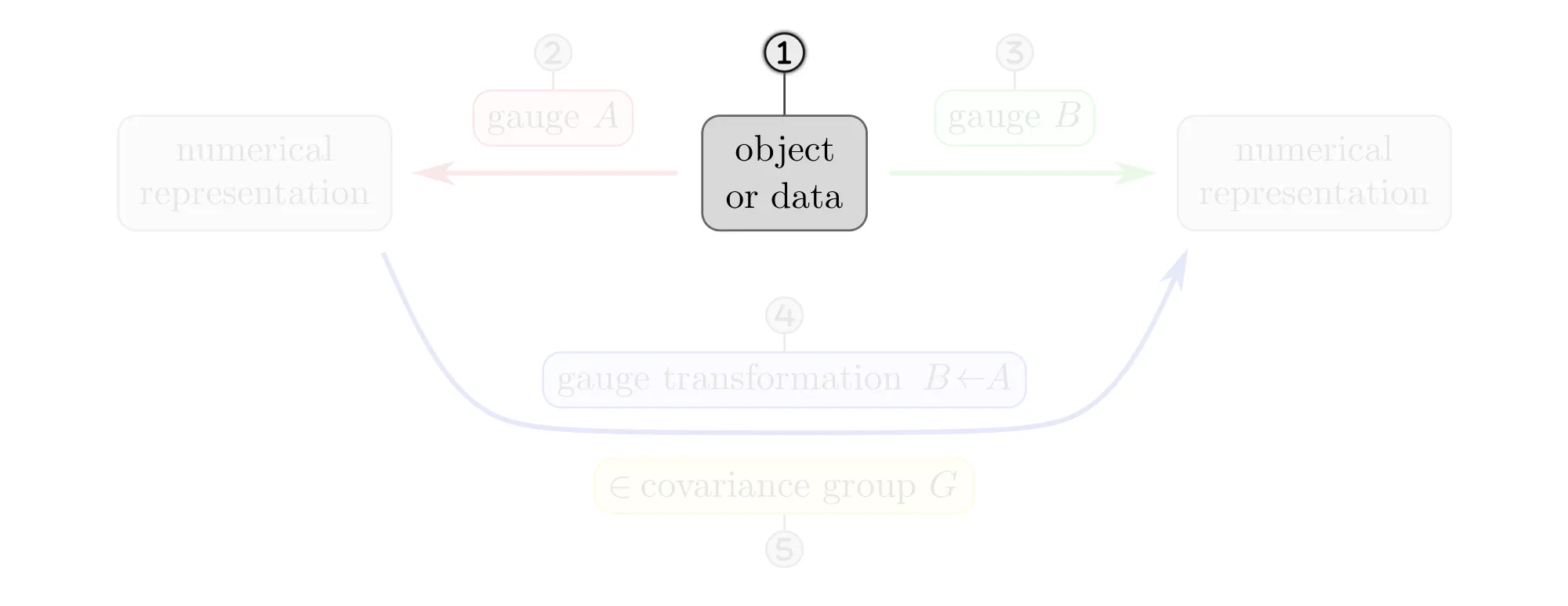
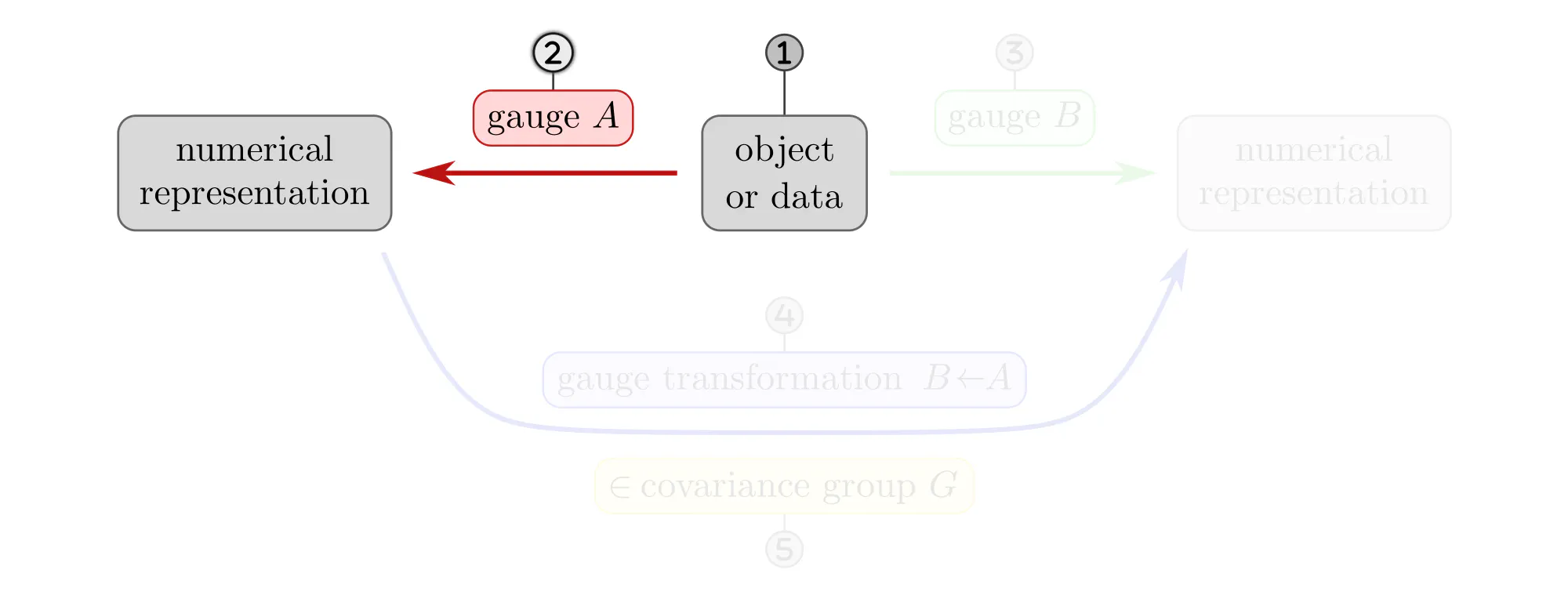
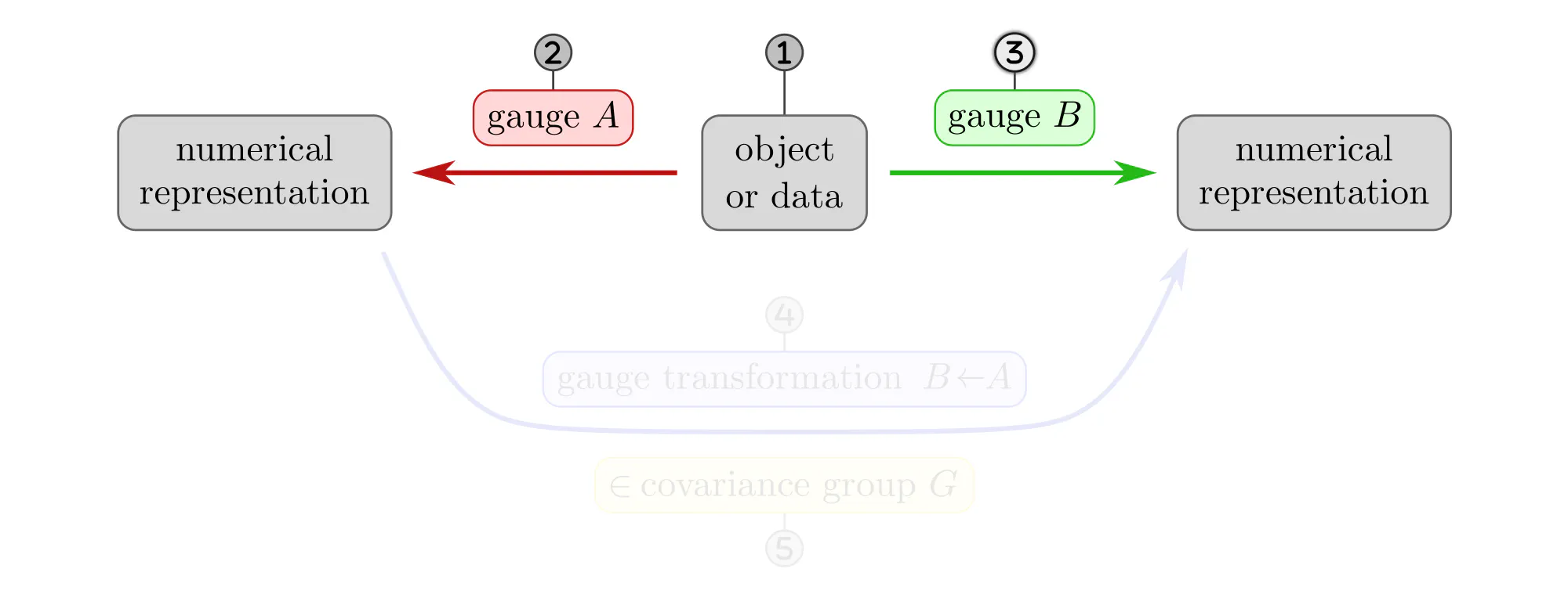
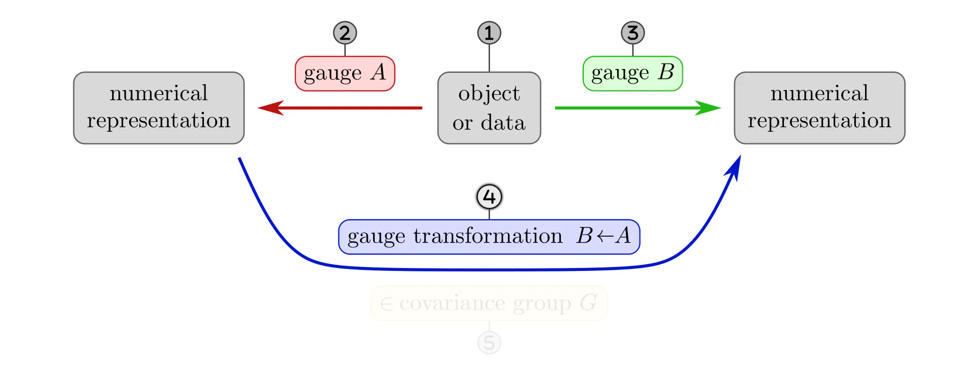
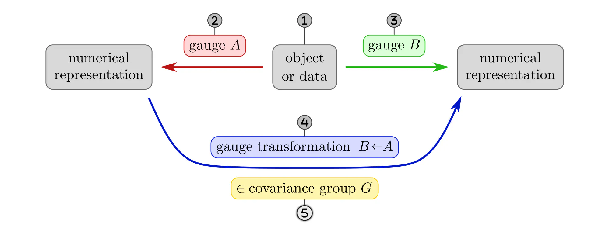
The following paragraphs clarify the concepts of gauges and gauge transformations with simple examples, like measuring distances, ordering set elements or the nodes of a graph, or assigning coordinates to Euclidean space. Each example will be explained as a different instantiation of the same abstract commutative diagram shown below. Click on the ❯ arrow to uncover the diagram and the explanatory bullet points step by step.

❮ ❯

There is some mathematical object or data that we would like to process using a neural network. A-priori, this object is not yet quantified or represented by concrete numerical data.
An example would be the wingspan of the dragonfly above, which exists independently from any concrete units of length.

The process of picking a concrete numerical representation is called gauging. The specific choice of representation is often ambiguous. We label gauges by capital Latin letters, e.g. gauge $A$.
For instance, the abstract wingspan could be quantified by a concrete number of centimeters.

Whenever there is no canonically preferred gauge, we have to consider alternative choices. To investigate the relationship between different gauges, we assume a second gauge, called gauge $B$.
Inches are another unit of length, representing the same abstract wingspan by different numbers.

The concrete numerical representations in different gauges are by definition equivalent (isomorphic), and one may always transform back and forth between them. Such conversions between equivalent data representations are called gauge transformations.
In our example, this would be a unit conversion from centimeters to inches, which is achieved by dividing the number of centimeters by the factor 2.54.

The ambiguity in the choice of gauges is naturally such that the gauge transformations between them form a group, which we call covariance group $G$. Some examples:

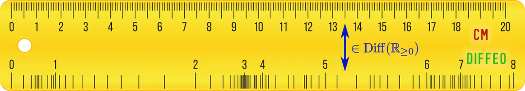
• Lengths are usually measured as multiples of some unit length, like centimeters or inches. Gauge transformations between different (positive) units of length are multiplications with positive numbers. They form the covariance group $G=(\mathbb{R}_{>0},\,\cdot\,)$.
• In principle, one would not have to measure lengths in "equidistant" units, but could use more general gauges such that the covariance group $G=\mathrm{Diff}(\mathbb{R}_{\geq0})$ consists of diffeomorphisms.
  
• If we can restrict to a single measurement unit, the covariance group becomes trivial, $G\!=\!\{e\}$.

Why should gauge transformations form a group in the first place? To clarify this question, note that the inherent ambiguity in picking gauges for an object comes from its symmetries. For instance, the identification of the circle below with numerical angles is only unique up to, e.g, rotations.

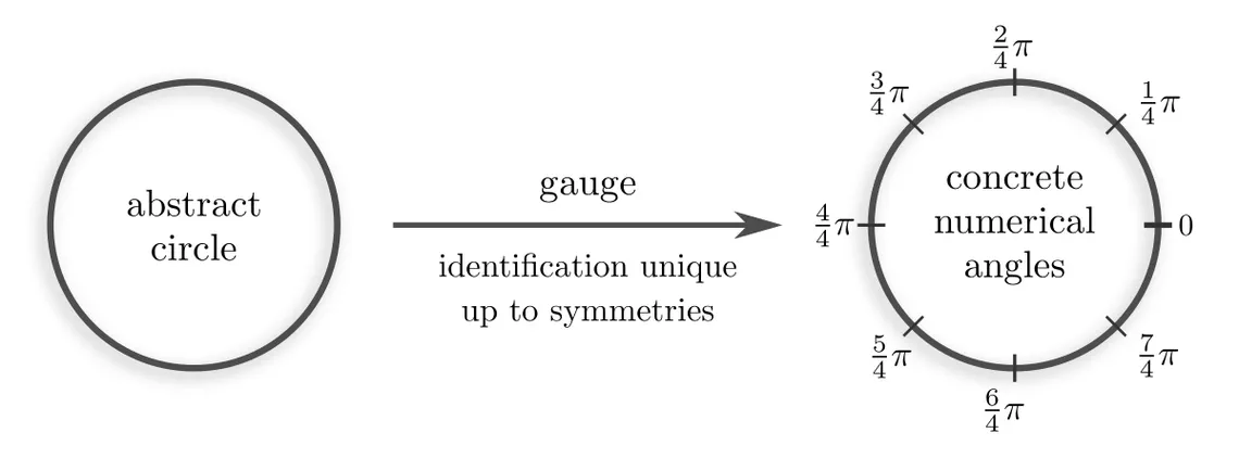
Rotations are just one example of what could be meant by “symmetries of a circle”. The specific level of symmetries of an object depends on the mathematical structure with which it is equipped. Let’s look at typical mathematical structures and the implied covariance groups for our example of gauging a circle.

In the context of deep learning, such $G$-ambiguities in the numerical representation of data need to be addressed by making neural networks $G$-covariant or $G$-equivariant. Before coming to equivariant networks, we give several examples of gauging data that is commonly appearing in deep learning applications.

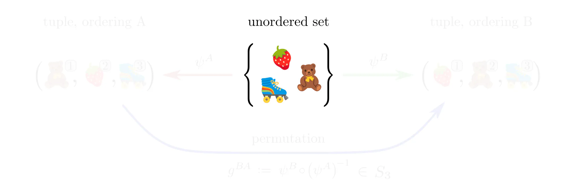
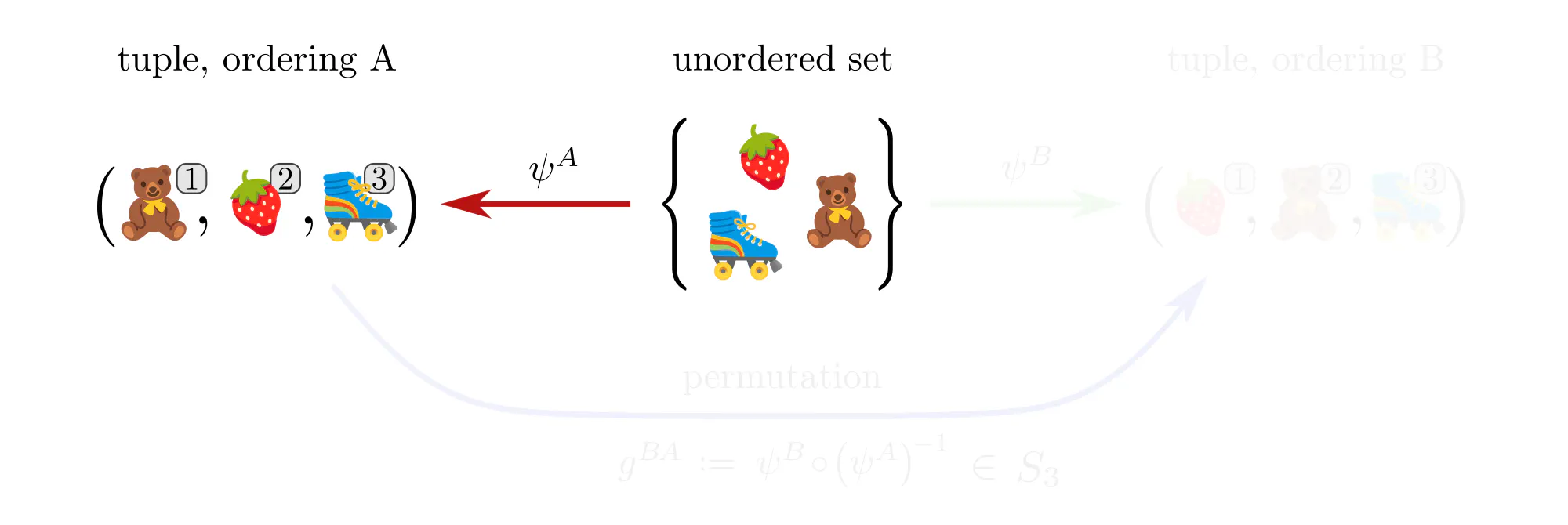
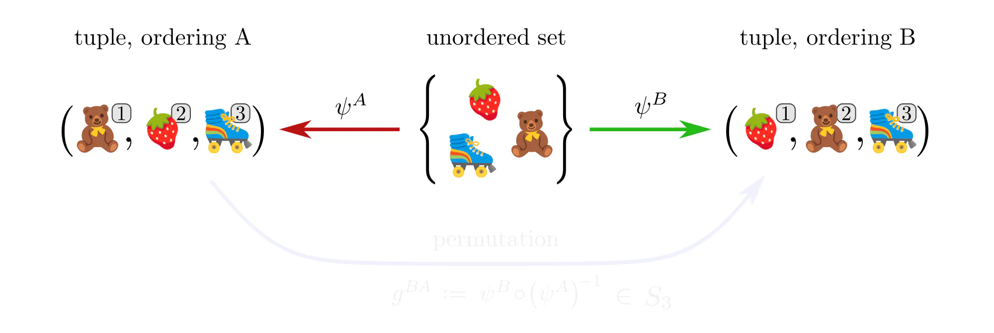
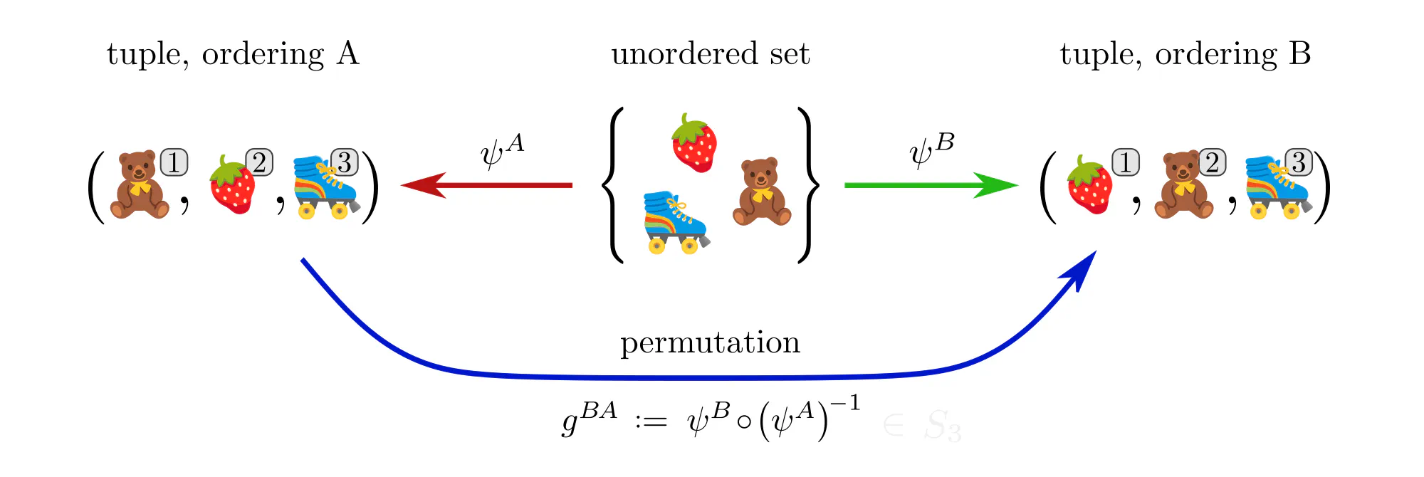
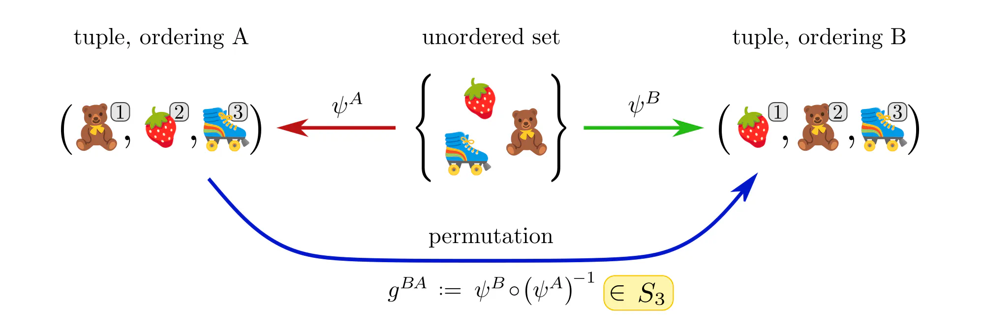
Example :  Ordering set elements

Data often comes in the form of sets (or multisets) of features without additional mathematical structure. Neural networks for such data, like the Deep Sets by (Zaheer et al., 2017), are typically permutation equivariant. Let’s see how these permutations arise in our gauge theoretic viewpoint.

❮ ❯

A set is a collection of elements without inherent ordering.

Numerically, a set is represented by some ordered tuple or array. The specific choice of ordering $A$ of set elements is the gauge-freedom of representing sets. Formally, the gauge is a choice of map $\psi^A: X \to \{1,\dots,N\}$ that assigns indices $1,\dots,N$ to elements of the set $X$.

A different gauge is simply a different choice of ordering $B$.

Gauge transformations are therefore permutations of ordered tuples.

A bare set does not have any mathematical structure that could reduce the choice of gauge to some subset of preferred element orderings. The covariance group is therefore the full symmetric group $G=S_N$, consisting of all  possible permutations.

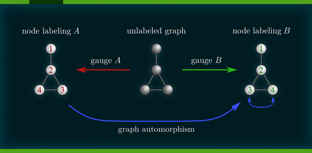
Example :  Labeling graph vertices

Graphs $\mathcal{G}=(V,E)$ are sets of vertices $V$, equipped with an additional edge structure $E \subseteq V\mkern-4mu\times\mkern-3muV$. This edge structure reduces the ambiguity of gauges such that gauge transformations take values in graph automorphisms (the symmetries of graphs) instead of more general vertex label permutations.

❮ ❯

A-priori, there is no canonical labeling or ordering of graph vertices given.

To represent graphs numerically, one needs to pick some vertex labeling $A$. As for bare sets, this labeling is given by a function $\psi^A: V \to \{1,\dots,|V|\}$. The specific choice of labeling determines the ordering of node or edge features, and of the rows and columns of adjacency matrices.

A different gauge is, of course, a different choice of vertex labeling $B$.

Gauge transformations are vertex label permutations. In practice, this would manifest in simultaneous permutations of node and edge features.

So far there was no difference to bare sets. However, the edge structure allows to reduce gauge transformations to graph automorphisms $G = \mathrm{Aut}(\mathcal{G})$ $\leq\, S_{|V|}$, i.e. those permutations that are symmetries of of the graph.

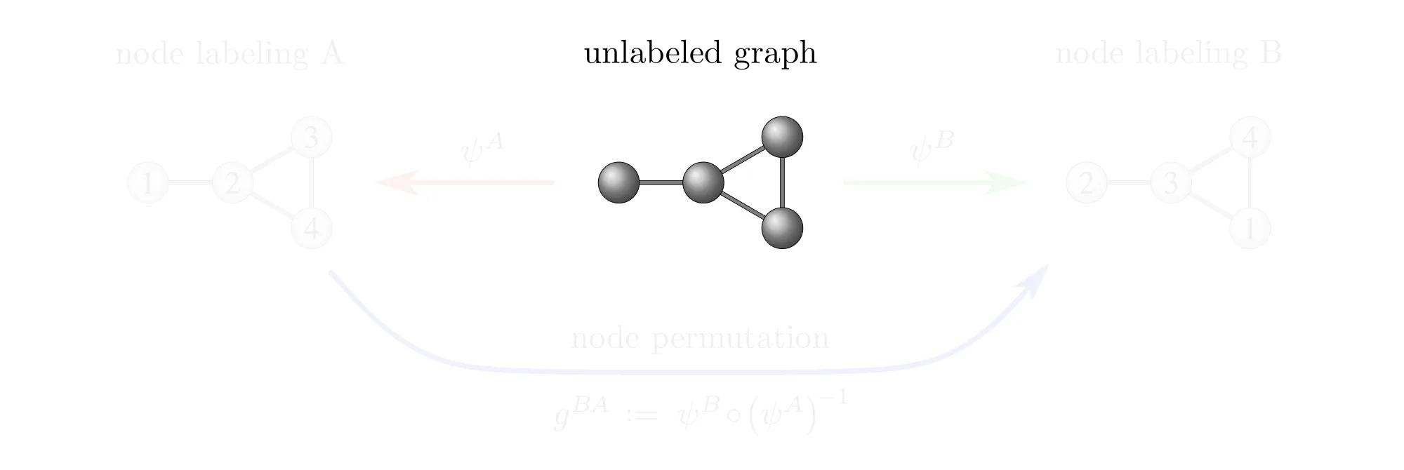
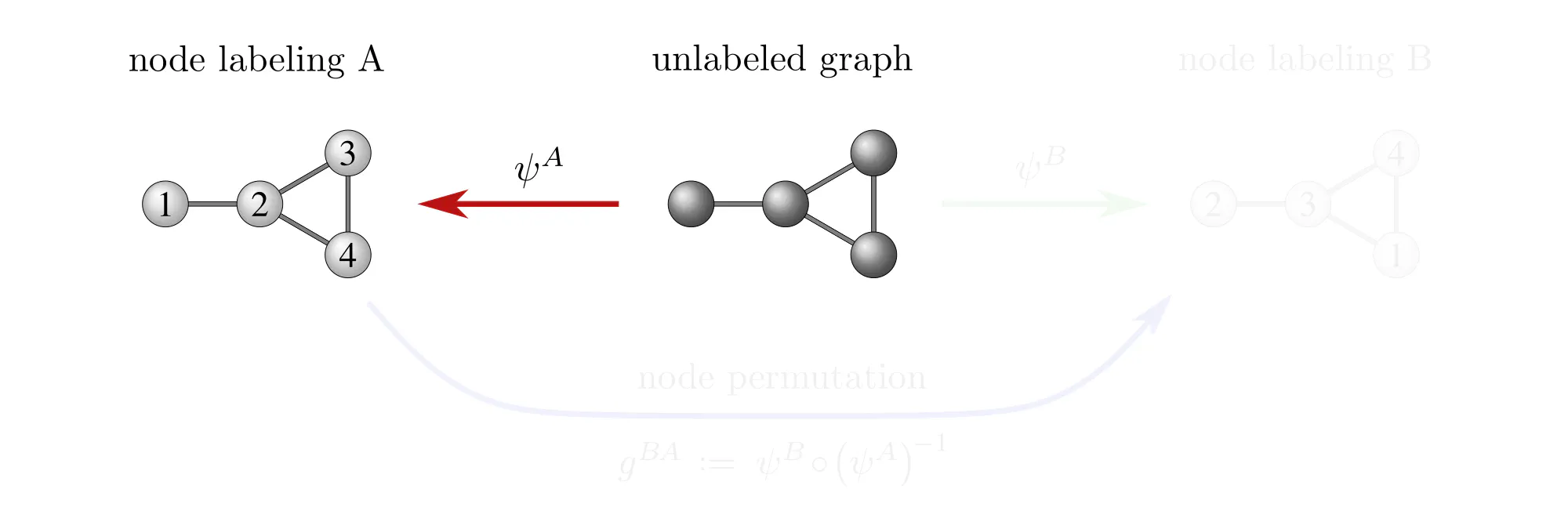
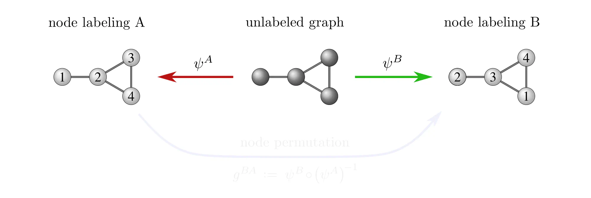
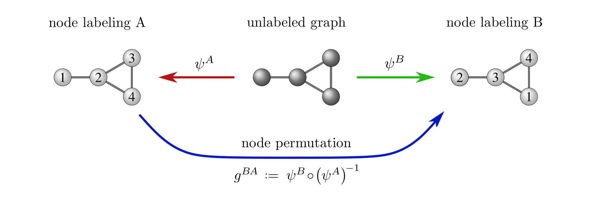
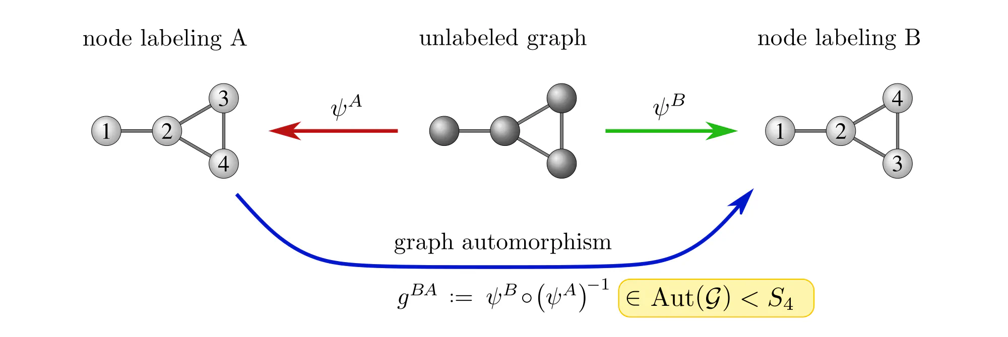
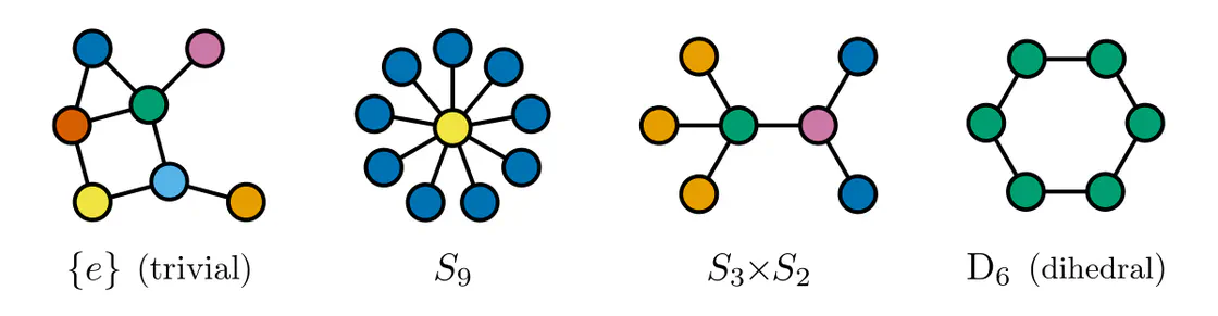
Some exemplary graphs and their automorphisms are shown below. Differently colored nodes are distinguished by their edge structure, while those of the same color remain indistinguishable. Gauges are accordingly disambiguated such that the remaining gauge transformations are only permutations within nodes of the same color. The simple graph in the slideshow above would only require two gauges, differing solely in how they assign the labels 3 and 4 to the two nodes on the right.

Some graph neural networks in the literature are fully permutation equivariant (Maron et al. 2019a), (2019b), while others are explicitly leveraging the edge structure, reducing equivariance to automorphisms (de Haan et al. 2020), (Thiede et al. 2021). From our gauge theoretic perspective, we interpret these models as different choices of covariance groups.

Example :  Assigning coordinates to Euclidean spaces

Convolutional neural networks (CNNs) process spatial signals, in the simplest case on Euclidean spaces. Gauges corresponds here to choices of coordinate systems, relative to which feature vector fields are represented numerically.

❮ ❯

When hearing "Euclidean space" you might think about Euclidean vector spaces $\mathbb{R}^d$. Here, we consider Euclidean affine spaces $\mathbb{E}_d$ instead, which lack the vector space structure. They have in particular no preferred choice of origin or coordinate system.

A gauge is a choice of (global) coordinate chart $A$. It is technically given by a map $x^A: \mathbb{E}_d \to \mathbb{R}^d$ which assigns the missing numerical coordinates $\mathbb{R}^d$ to the coordinate free Euclidean space $\mathbb{E}_d$.

Any other coordinate chart $B$ represents the same points in $\mathbb{E}_d$ by alternative coordinates in $\mathbb{R}^d$.

The coordinate vectors assigned by two different charts are related by chart transition maps, i.e. functions $x^{B}\circ(x^A)^{-1}: \mathbb{R}^d\to\mathbb{R}^d$.

The specific group to which transition maps are restricted depends on the geometric structure with which we assume the Euclidean space $\mathbb{E}_d$ to be equipped:

• As $\mathbb{E}_d$ has an affine structure, we can take charts to be affine maps. This implies gauge transformations which take values in the (general) affine group $\mathrm{Aff}(\mathbb{R}^d)$ of $\mathbb{R}^d$.
• Assuming e.g. an additional metric structure, we can restrict to distance-preserving charts and transition maps, i.e. isometries. The corresponding covariance group is the isometry group of $\mathbb{R}^d$, called Euclidean group $\mathrm{E}(d)$. Adding an orientation to $\mathbb{E}_d$ allows to reduce this further to the special Euclidean group $\mathrm{SE}(d)$.
• When the geometric structure of $\mathbb{E}_d$ allows in addition to distinguish "up" and "down" directions, we end up with pure translations $(\mathbb{R}^d,+)$ of $\mathbb{R}^d$.
• Gauge transformations become trivial, $G=\{e\}$, when $\mathbb{E}_d$ is uniquely identified with $\mathbb{R}^d$, which additionally requires some point to be selected as origin.
• As a last example, consider the Euclidean space $\mathbb{E}_d$ as smooth or topological manifold, forgetting about the affine structure. As probably already guessed, the corresponding gauge transformations are diffeomorphisms in $\mathrm{Diff}(\mathbb{R}^d)$ or homeomorphisms in $\mathrm{Homeo}(\mathbb{R}^d)$.

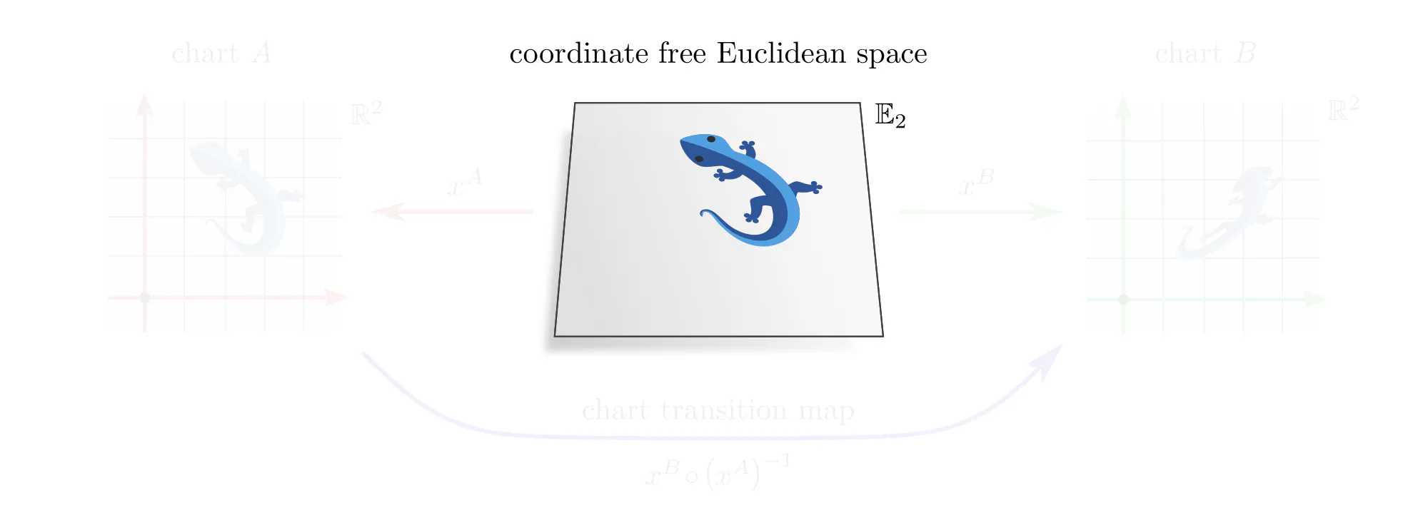
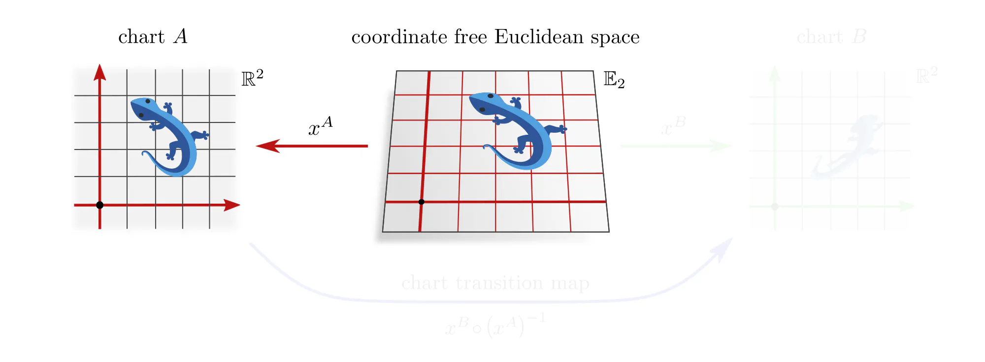
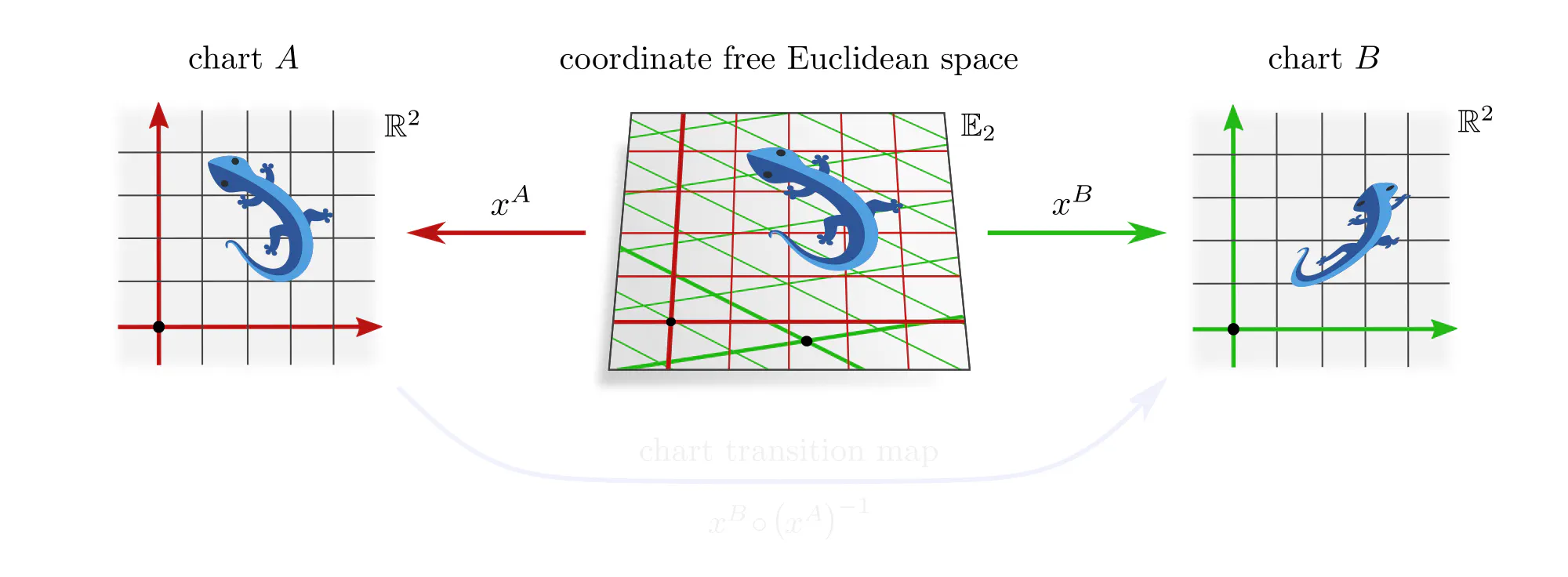
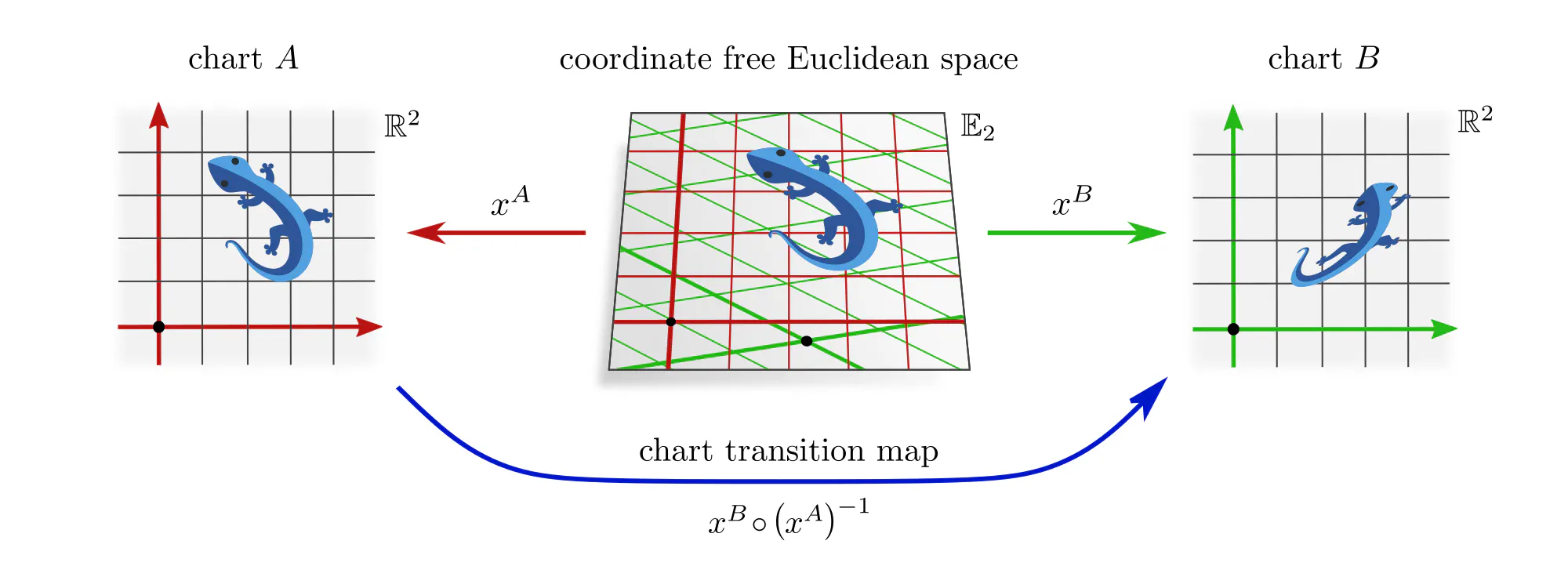
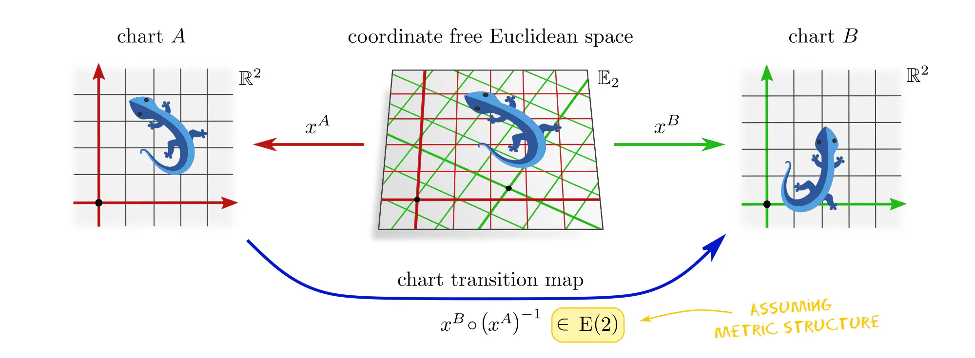
If you never thought about choices of coordinate charts in the context of convolutional networks, this is since numerical samples are usually already expressed in some gauge. In practice, this choice of chart would find expression in the specific pixel grid of an image or the coordinates of a point cloud. In the case of photos, it is the photographer who selects a gauge by picking some camera alignment relative to the scene.

When processing such data, it is important to ask in how far the choice of gauge was canonical. In the forest photo below, the photographer aligned their camera horizontally, which is canonically possible due to the preferred “up/down” direction implied by gravity. However, for aerial or microscopy images, the camera rotation is arbitrary, i.e. represents just one of a whole set of equivalent gauges.

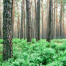
As explained in the following section, such gauge ambiguities need to be addressed by “gauge equivariant” neural networks.

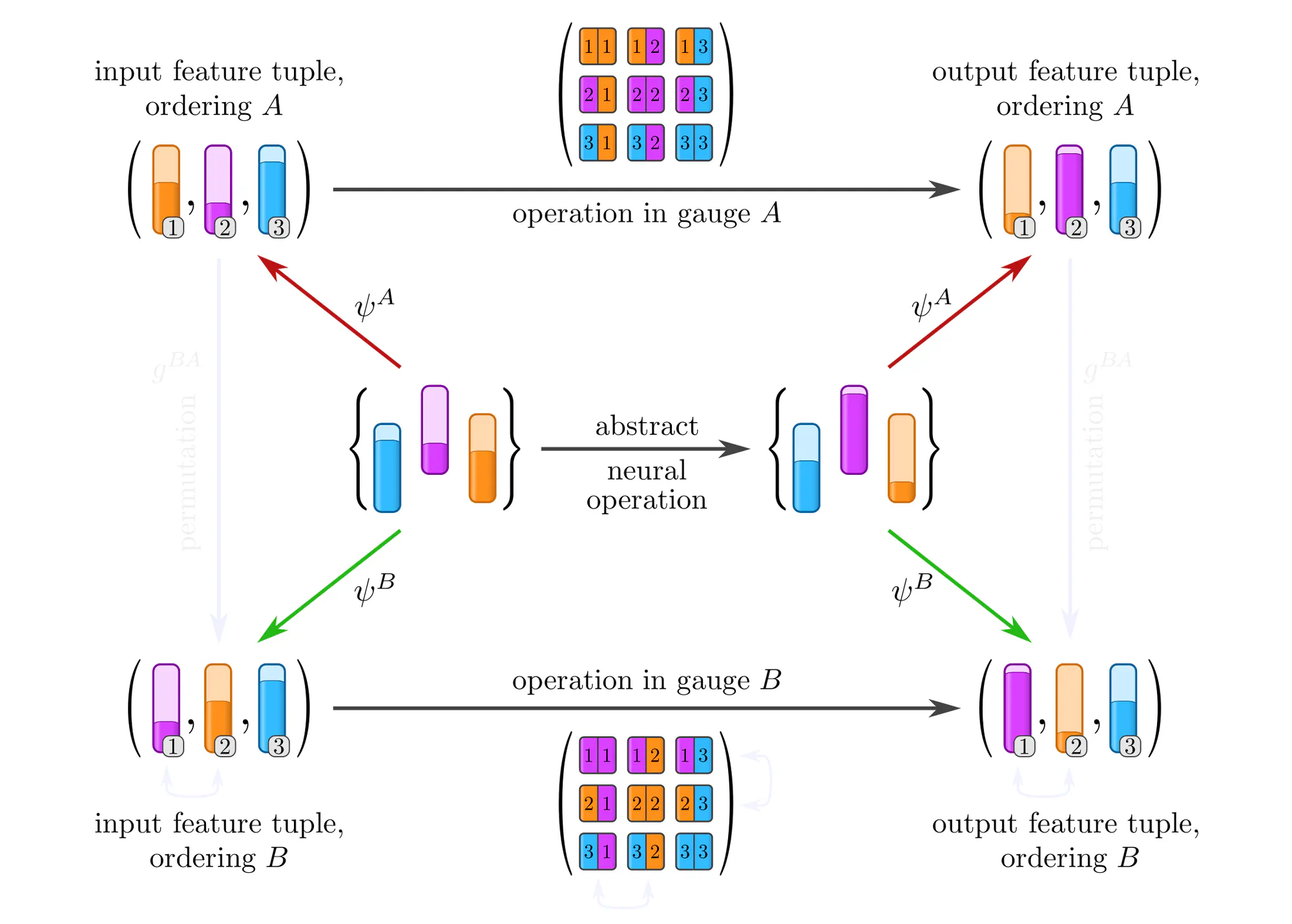
So far, we discussed gauges and gauge transformations of data or other mathematical objects. We turn now to the gauging of neural network layers, i.e. of the functions that map between data  (morphisms). Just as for the data itself, concrete numerical representations of an abstract neural operation will (in general) differ among gauges, and are related by gauge transformations. The specific choice of gauge is ultimately arbitrary, since the outputs of such numerical representations of network layers are guaranteed to transform as expected under gauge transformations.

It is important to distinguish two closely related concepts:

• Covariance refers to the consistency of a mathematical theory under gauge transformations. All computations, i.e. all objects and morphisms, can be expressed in any gauge.
• Equivariance is a stronger condition which imposes symmetry constraints on network layers. It can either be understood as the property of the layer to commute with (gauge)transformations, or, equivalently, as the invariance of the layer's numerical representation under (gauge)transformations.

The next paragraphs clarify what it means for a network layer to be covariant. After that, we explain how this relates to equivariant layers, when or why equivariance is actually required, and how it relates to Einstein’s theory of relativity.

Covariant network operations

The principle of covariance has a long history in physics, usually referring specifically to the coordinate independence of a theory. Albert Einstein (1916) formulated it as follows:

“Universal laws of nature are to be expressed by equations which hold good for all systems of coordinates, that is, are covariant with respect to any substitutions whatever.”

Adapted to machine learning and to more general data gauges, this principle becomes:

“Machine learning models are to be expressed by equations which hold good for all numerical data representations, that is, are covariant with respect to any gauge transformations.”

This is best explained with a few examples.

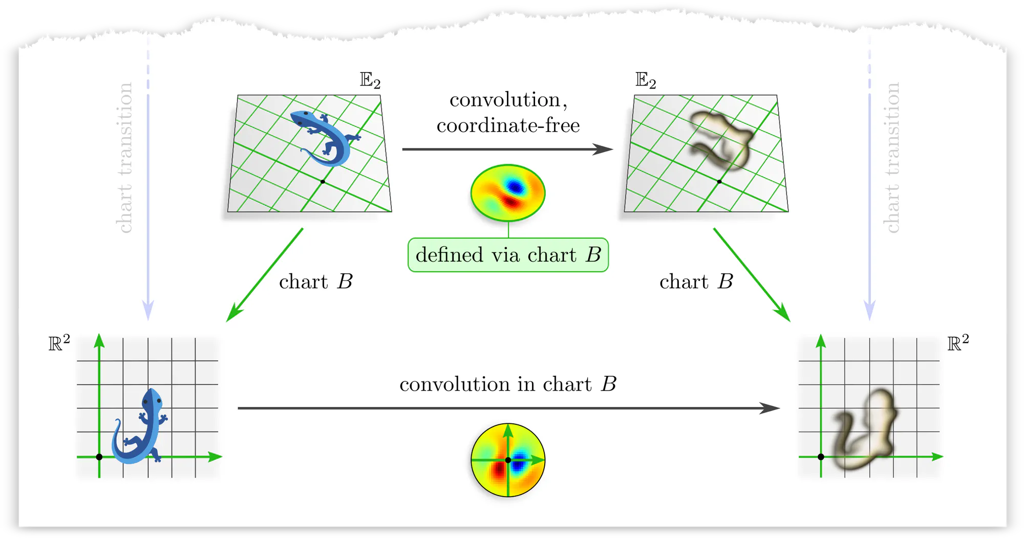
Example :  Covariant convolutions

As it is geometrically very intuitive – almost tautological – our first example is that of a convolution layer, which can be expressed in different coordinate charts.

❮ ❯

Convolution layers map input feature fields to output feature fields by convolving them with some kernel. This operation exists independently from any choice of coordinates.

To implement it numerically, the feature fields are both expressed in some chart $A$. The commutativity of the diagram implies the coordinate expression $$\mathrm{conv}^A\ :=\ \mathrm{chart}^A \circ \mathrm{conv}^{\times} \circ \big(\mathrm{chart}^A\big)^{-1}$$ of the convolution in terms of the coordinate free operation $\mathrm{conv}^{\times}$ and the charts.

One could of course have used any other chart $B$ instead, implying an alternative coordinate expression $\mathrm{conv}^B$, which corresponds to expressing the kernel in different (e.g. rotated) coordinates. This is an alternative numerical representation of the same abstract operation.

As already seen above, charts $x^A$ and $x^B$ imply transition maps :  $\mathrm{transition}^{BA} := x^B \mkern-2mu\circ\mkern-2mu (x^A)^{-1}\mkern-2mu.$

The commutativity of the outer square implies the covariant transformation law $$ \mathrm{conv}^B\ =\ \mathrm{transition}^{BA} \circ \mathrm{conv}^A \circ \big(\mathrm{transition}^{BA}\big)^{-1}, $$ which relates different coordinate expressions of the convolution layer.

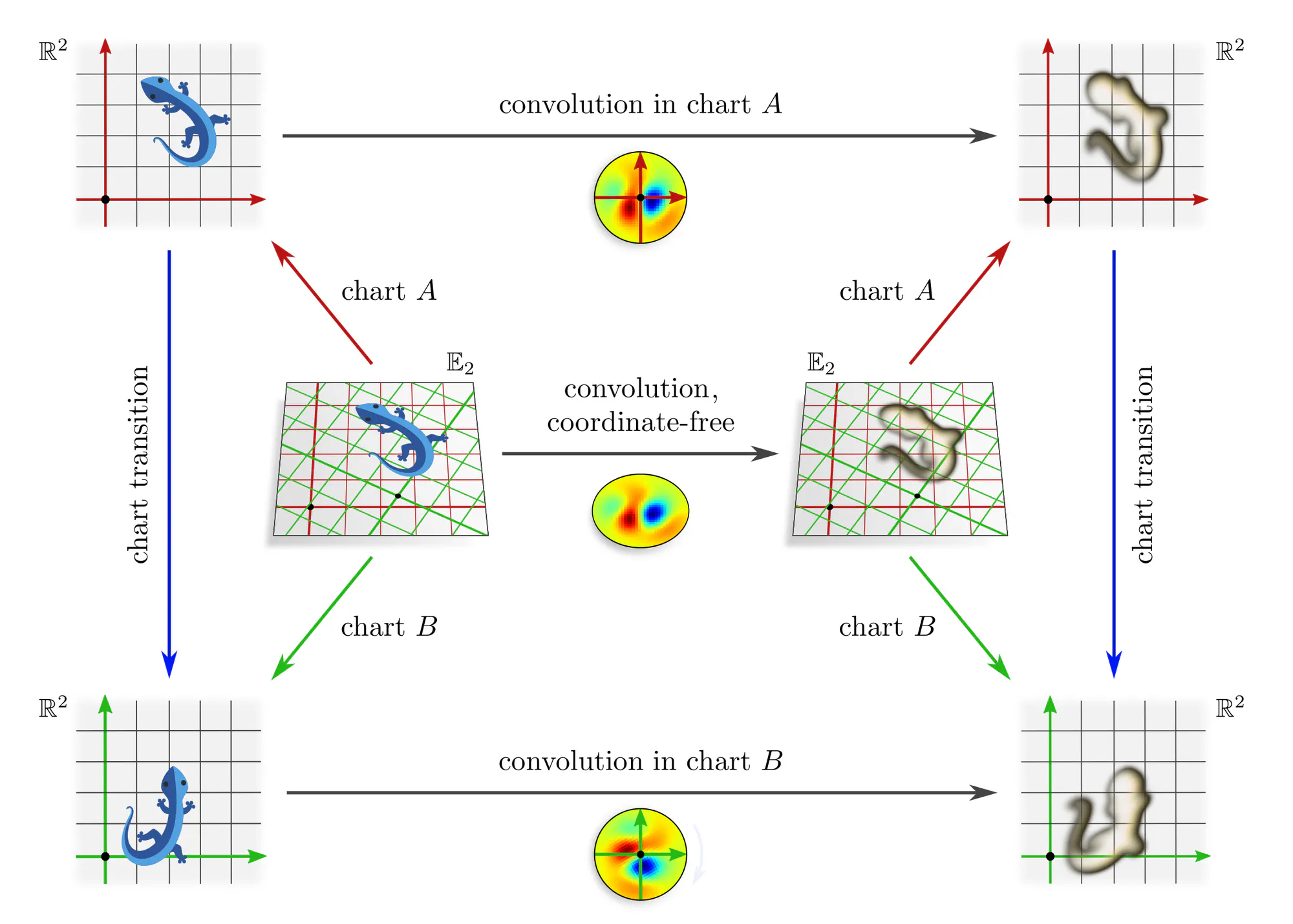
Note that covariance merely explains how different coordinate expressions $\mathrm{conv}^A$ and $\mathrm{conv}^B$ of the convolution relate, but does not require any constraints on the convolution itself! The outer commutative square is in particular not an equivariance diagram, as this would require that the top and bottom arrows are the same (invariant) operation. The corresponding equivariance diagram is discussed further below.

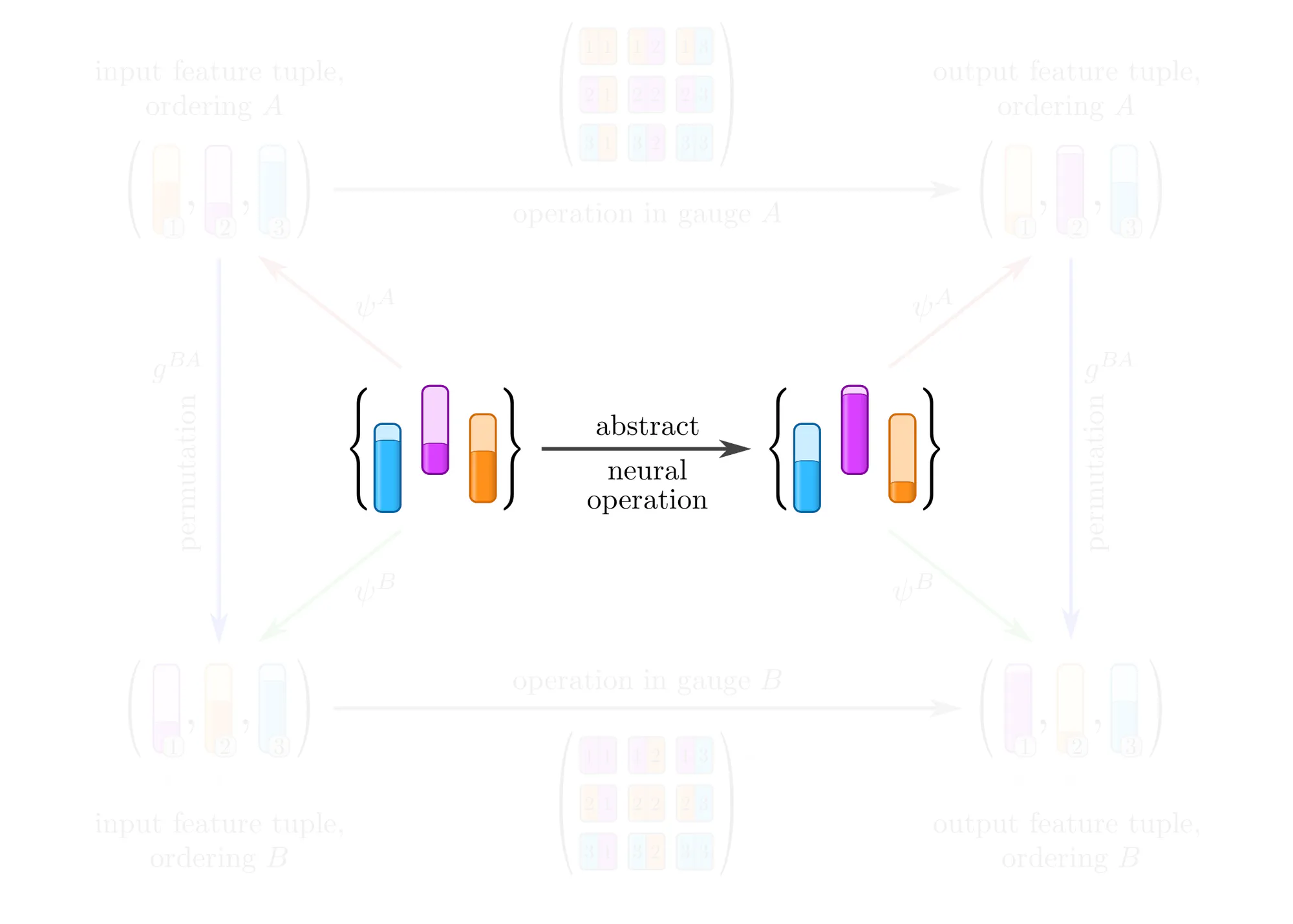
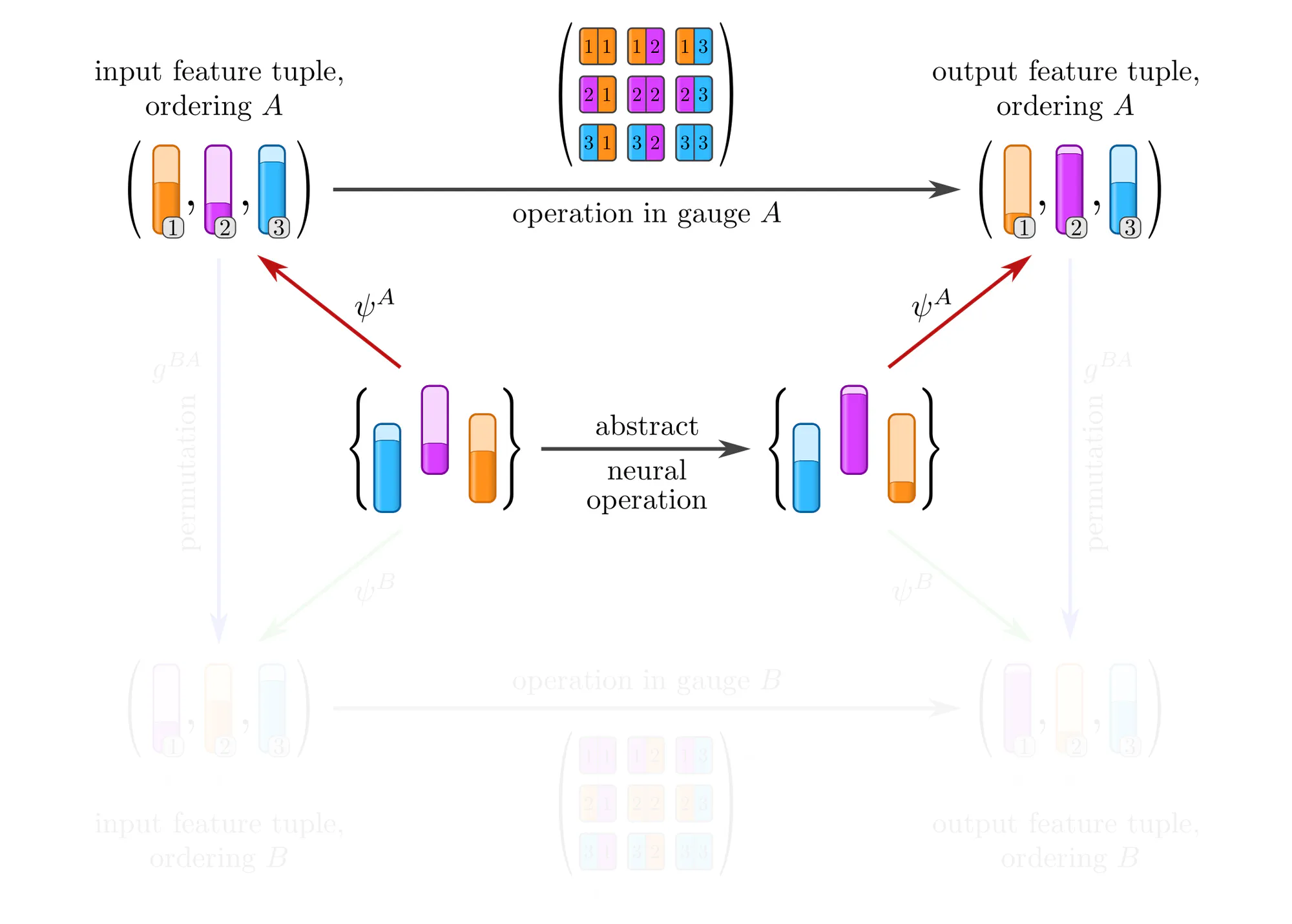
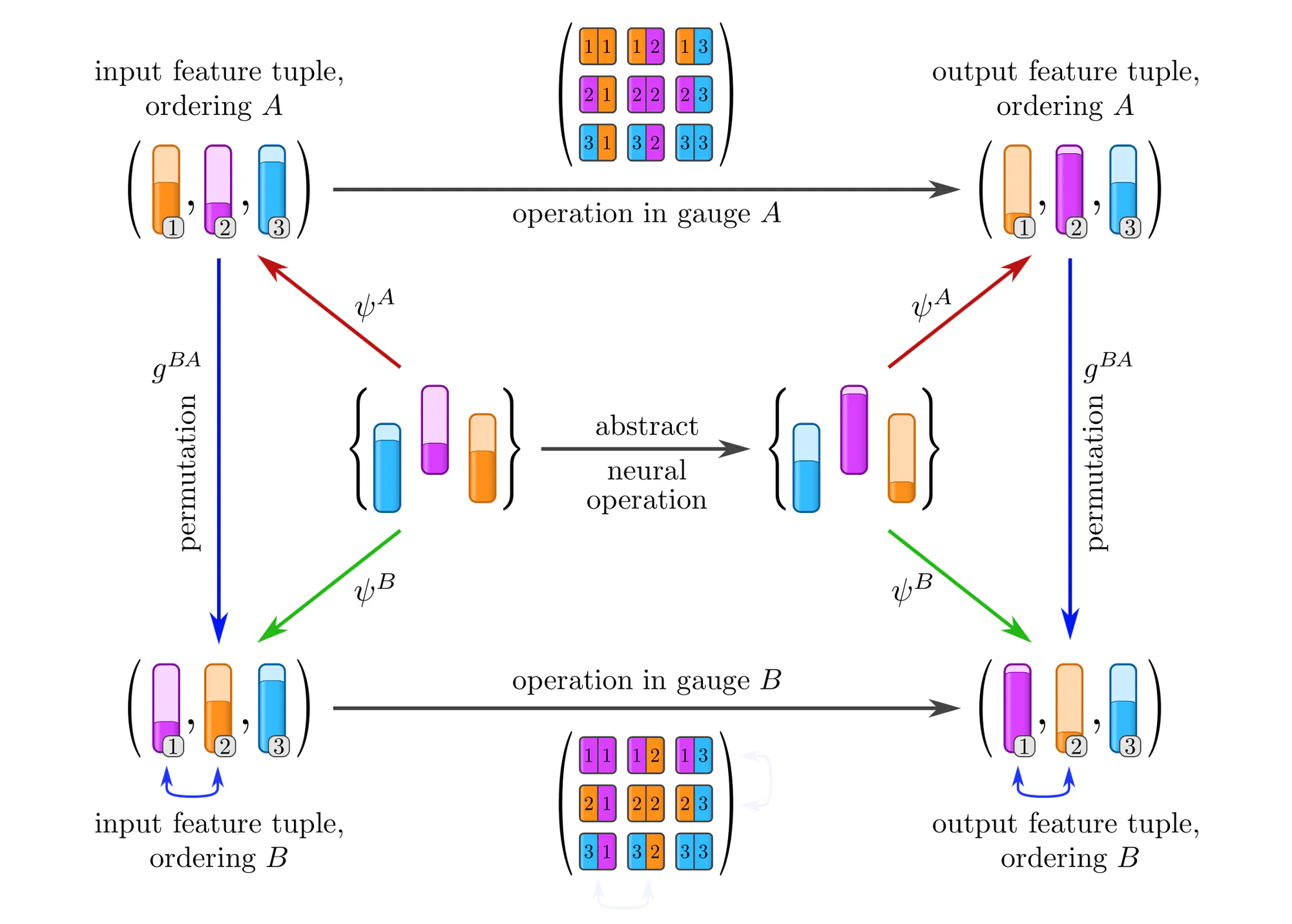
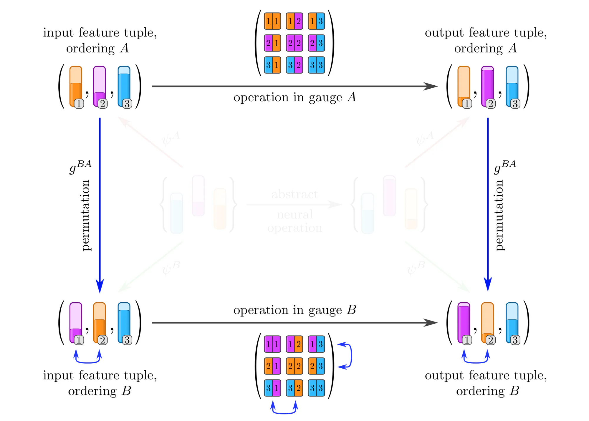
Example :  Covariant operations on sets of features

Analogous considerations apply to the other examples above, for instance to layers that map between unordered sets of feature vectors.

❮ ❯

Layers that map between sets of feature vectors are well-defined without referring to a particular ordering of the features.

However, a numerical implementation will represent the sets as tuples in some ordering $A$. This implies, again, a concrete numerical representation of the abstract operation.
The visualization shows the example of a linear operation, which would linearly accumulate input features into output features via a matrix of weights in the chosen ordering.

Alternative orderings $B$ imply different yet equivalent numerical representations of this operation.

The tuples of features are related by permutations $g^{BA} := \psi^B \circ \big(\psi^A \big)^{-1}$.

The covariant transformation law between the layer's expression in different gauges is given by a pre and post-composition with permutations of features: $$\mathrm{operation}^B\ =\ g^{BA}\circ \mathrm{operation}^A \circ \big(g^{BA} \big)^{-1}$$ In the visualized example, this would be a permutation of the matrix rows and columns. Note the similarity to the (covariant) transformation of a matrix under a change of basis, e.g. in an eigendecomposition.

Equivariant network operations

In the above analysis we assumed some abstract operation to be given (the middle horizontal arrow), and studied its numerical representations in various gauges (the top and bottom horizontal arrows). In practice, the situation is insofar different that we are rather given a concrete numerical operation, e.g. a kernel or weight matrix optimized on previous samples, and need to apply it to the next sample. The fundamental issue here is that the gauges that we could pick to represent this next sample are inherently arbitrary, and that

applying a given (fixed) numerical operation in different gauges yields in general different results!

The usual naive “solution” is to ignore the arbitrariness, and simply go ahead with the specific gauge in which the sample happens to be stored in the dataset. A clean solution should instead respect the structural equivalence of gauges  –  as we will see, this leads to gauge equivariant operations.

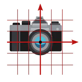
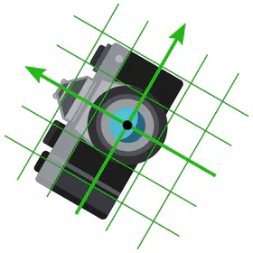
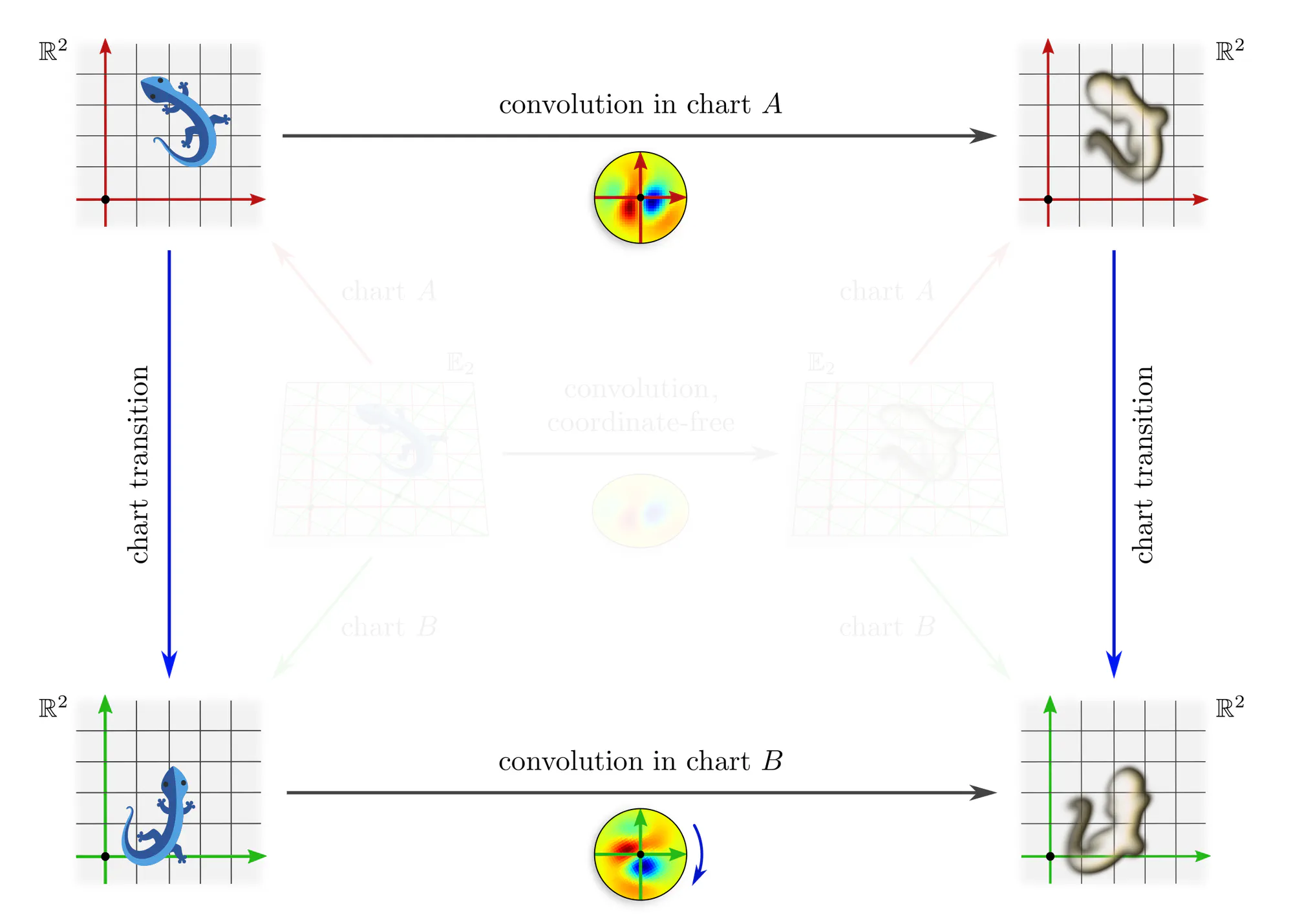
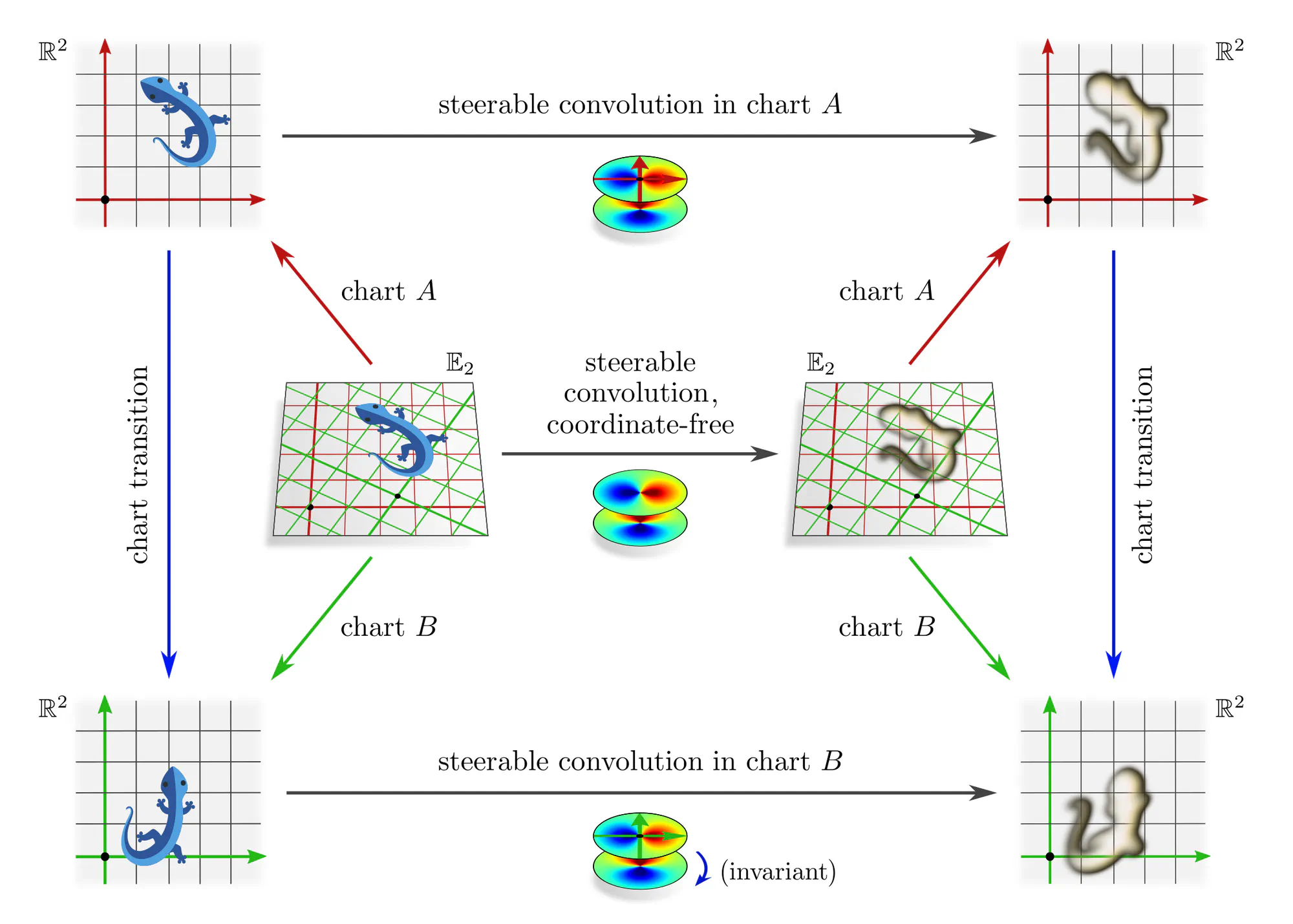
(Counter)Example :  Applying a kernel in different charts

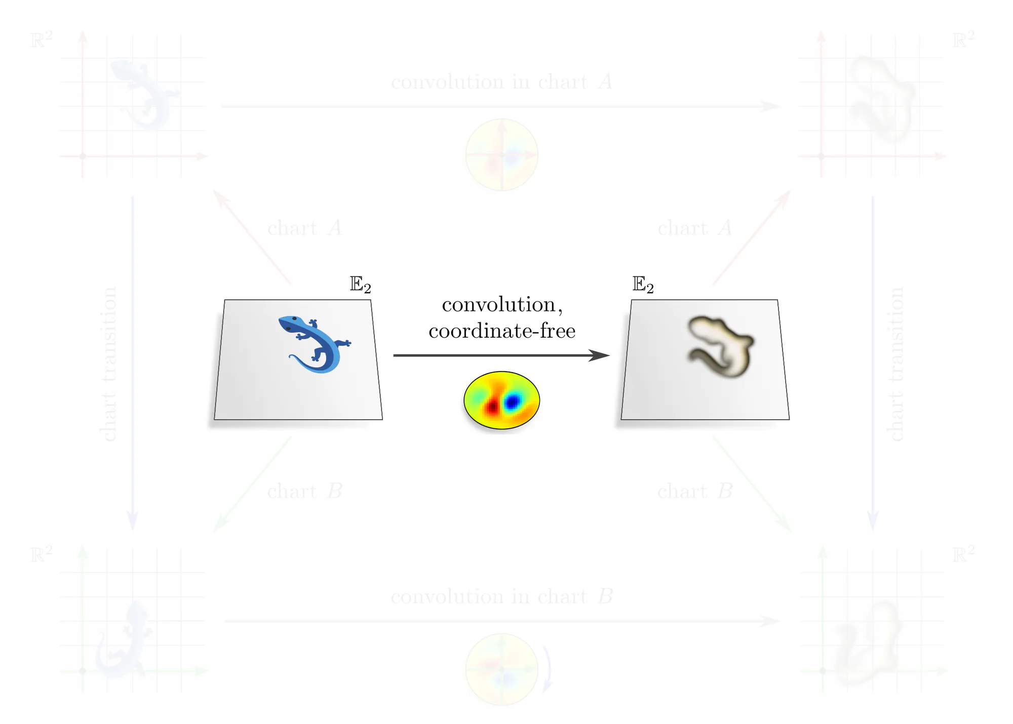
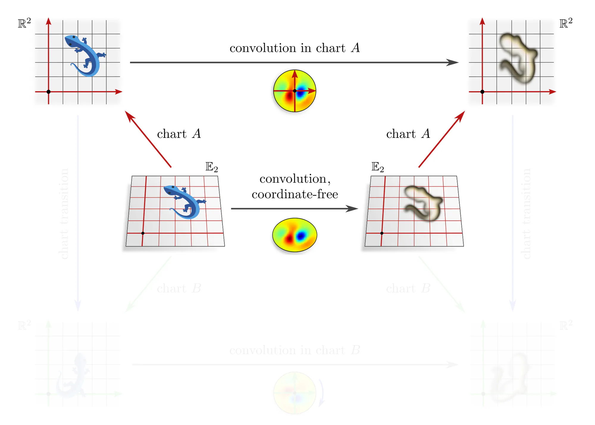
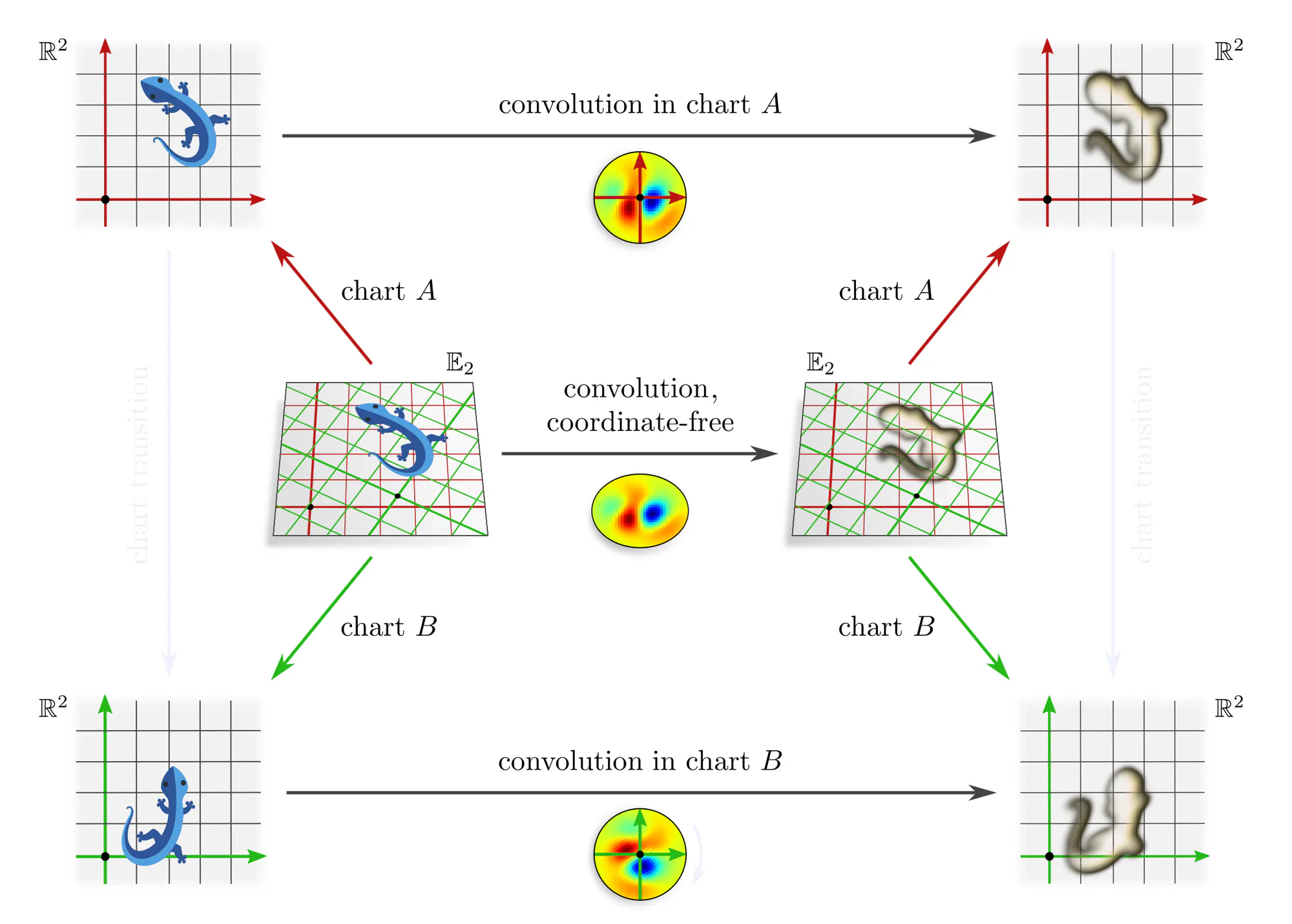
Let’s get back to the concrete example of convolutions to make this issue more intuitive. Assume that we are given a learned numerical kernel . We apply it to an image, which the photographer arbitrarily decided to shoot in some chart $A$. This concrete numerical operation, given by the top horizontal arrow in the diagram below, implies the corresponding abstract convolution operation given by the bottom horizontal arrow.

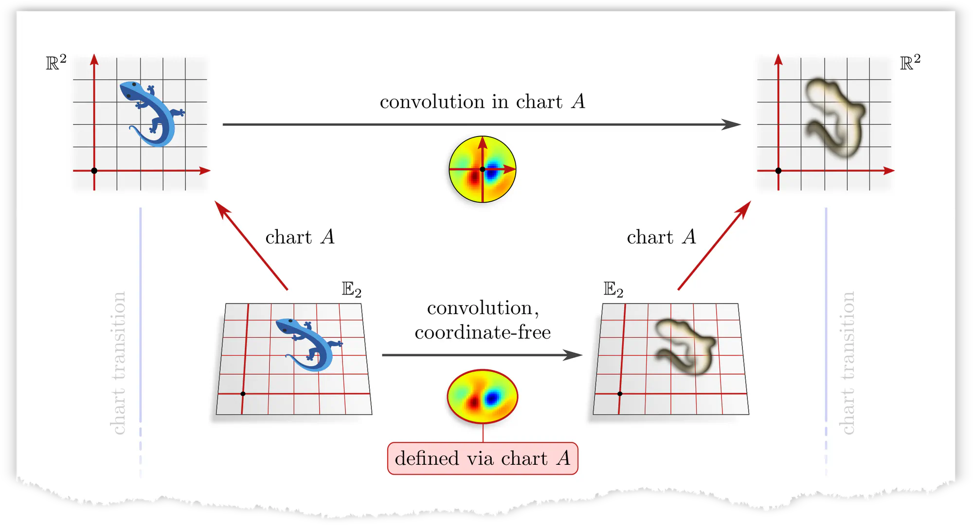
However, the photographer could equally well have chosen any other camera alignment aka chart $B$. Applying the kernel in this gauge instead implies a different abstract convolution operation with a correspondingly transformed kernel.

The issue is that applying the kernel in any particular chart breaks the structural equivalence of gauges. To prevent this, we need to find a way to apply the kernel in such a way that all gauges are treated equivalently.

How can the equivalence of gauges be preserved? Denoting the given numerical operation that we would like to apply by $\widetilde{\mathrm{op}\vphantom{\rule{0pt}{5.2pt}}}$, we either assigned $$ \mathrm{op}^A\ :=\ \widetilde{\textup{op}\vphantom{\rule{0pt}{5.2pt}}} \mkern40mu\textit{or}\mkern40mu \mathrm{op}^B\ :=\ \widetilde{\mathrm{op}\vphantom{\rule{0pt}{5.2pt}}}\mkern2mu, $$ thus arbitrarily preferring one of the gauges $A$ or $B$. Such symmetry breaking choices can be avoided by assigning $\widetilde{\mathrm{op}\vphantom{\rule{0pt}{5.2pt}}}$ to all gauges simultaneously, implying in particular $$\mathrm{op}^A\ =\ \mathrm{op}^B\ :=\ \widetilde{\textup{op}\vphantom{\rule{0pt}{5.2pt}}}$$ for any two gauges $A$ and $B$. One may think about this approach as a form of parameter sharing across gauges, or as the invariance of the operation’s numerical representations under gauge transformations.

An immediate consequence of this parameter sharing across gauges is that $\widetilde{\mathrm{op}\vphantom{\rule{0pt}{5.2pt}}}$ needs to be equivariant under gauge transformations. To derive this result, recall that the numerical expressions of an operation in two gauges are related by: $$\mkern{93mu} \mathrm{op}^B\ =\ g^{BA}\,\circ\, \mathrm{op}^A \,\circ\, \big(g^{BA}\big)^{-1} \mkern57mu(\textit{co}\textup{variance}) $$ Substituting $\mathrm{op}^A$ and $\mathrm{op}^B$ with the shared operation $\widetilde{\mathrm{op}\vphantom{\rule{0pt}{5.2pt}}}$ implies a gauge equivariance constraint : $$\begin{align} \widetilde{\mathrm{op}\vphantom{\rule{0pt}{5.2pt}}} \ &=\ g^{BA}\,\circ\, \widetilde{\mathrm{op}\vphantom{\rule{0pt}{5.2pt}}} \,\circ\, \big(g^{BA}\big)^{-1} \\[6pt] \iff\mkern40mu \widetilde{\mathrm{op}\vphantom{\rule{0pt}{5.2pt}}} \,\circ\, g^{BA} \ &=\ g^{BA}\,\circ\, \widetilde{\mathrm{op}\vphantom{\rule{0pt}{5.2pt}}} \mkern{150mu}(\textit{equi}\textup{variance}) \end{align}\mkern{20mu} $$ The relation between covariant and equivariant operations is concisely summarized by their commutative diagrams:

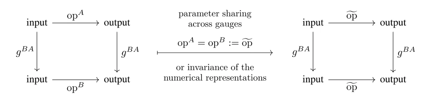
Intuitively, one may apply a gauge equivariant operation $\widetilde{\mathrm{op}\vphantom{\rule{0pt}{5.2pt}}}$ in any choice of gauge $A$ without breaking the structural equivalence of gauges: When $\widetilde{\mathrm{op}\vphantom{\rule{0pt}{5.2pt}}}$ is applied in any other gauge $B$, the resulting features are guaranteed to transform by $g^{BA}$, i.e. they are covariant (gauge independent).

Example :  Transition map equivariant convolutions

Let the gauges again be charts that assign coordinates to Euclidean space and let the chart transition maps be affine transformations $\mathrm{Aff}(G)$. Any numerical operation whose responses should be equivalent (covariant) when applying it in different charts needs to be $\mathrm{Aff}(G)$-equivariant. This brings us back to the steerable CNNs from the previous post. For instance, any coordinate chart independent linear map is necessarily a convolution with a $G$-steerable kernel.

An advantage of the gauge theoretic viewpoint is that it clarifies how equivariant networks imply a consistent coordinate free operation. More importantly, only this viewpoint extends to convolutions on more general manifolds and to local gauge transformations (gauge fields).

Other examples of (gauge) equivariant operations, which may be applied in arbitrary gauges, are Deep Sets (Zaheer et al., 2017) or the models of (Maron et al. 2019a), (2019b) for full permutation equivariance, or the graph neural networks by (de Haan et al. 2020) and (Thiede et al. 2021) for graph automorphisms. They correspond to similar commutative diagrams as that in the previous example.

On equivariance and relativity

The considerations in this post show remarkable analogies to Einstein’s theory of relativity. A physical theory should be covariant in the sense that any physical quantity and the system dynamics should be expressible in arbitrary coordinates. We apply the same principle of covariance to more general data and functions.

It is often emphasized that the principle of covariance is merely a statement about the mathematical formulation of physics (its coordinate independence), but does not impact the laws of nature themselves. Similarly, covariant network layers are consistently expressed in different gauges, but are themselves not constrained.

The special principle of relativity requires that the laws of nature take the same form in all inertial frames of reference, i.e., that they are invariant under Lorentz (or Poincaré) transformations. A simple example is the metric $\eta$ of Minkowski space, which takes the same form $\eta^A = \eta^B = \widetilde{\eta} := \mathrm{diag}(1,-1,-1,-1)$ in any inertial frames $A$ or $B$. Our analog are gauge equivariant network operations, which take the same invariant expression $\mathrm{op}^A = \mathrm{op}^B = \widetilde{\textup{op}\vphantom{\rule{0pt}{5.2pt}}}$ in any gauges. The invariant laws of nature correspond similarly to an equivariant system dynamics in the sense that Lorentz transformed initial conditions result in accordingly transformed evolved states.

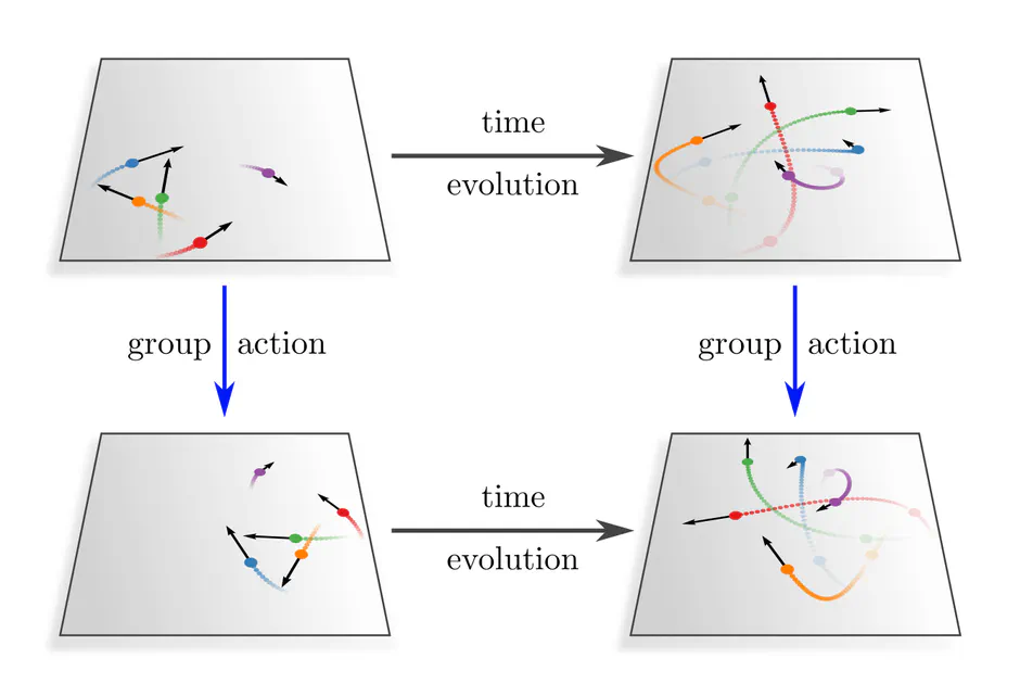
In physics, the invariance of the laws of nature implies that an experimenter can only perform relative measurements. $G$-equivariant network layers in deep learning are similarly only sensitive to the $G$-relative pose of feature vectors. For instance, one of our theorems requires that convolutional network features depend only on the relative distance between features but not on their absolute position.

The main takeaways of this post are:

• Numerical representation of data are not necessarily unique. A specific choice among the equivalent numerical representations is called gauge. Formally, gauges are choices of non-canonical isomorphisms $\psi^X: D \to R$ from the data $D$ to a numerical reference object $R$.
• Gauge transformations $g^{BA} := \psi^B \mkern-2mu\circ\mkern-2mu (\psi^A)^{-1}:\ R\to R$ allow to transform back and forth between different numerical representations $A$ and $B$.
• In how far gauges are ambiguous depends on the mathematical structure of the data. The level of ambiguity is captured by the covariance group $\boldsymbol{G}$, consisting of all gauge transformations. This group may be larger, but can not canonically be reduced beyond the symmetries of the data.
• Gauges do not only fix the numerical representation of data (objects), but also of neural network layers (morphisms). The consistent transformation behavior of a theory is referred to as covariance. Covariance does not imply a constraint on the network layers, but only their gauge independence.
• Given a numerical operation, it is unclear in which of the equivalent gauges it should be applied. When the output of the operation should be independent form the specific choice of gauge, i.e. transform covariantly, the operation needs to be equivariant under gauge transformations. This result explains common equivariant networks from a novel viewpoint.
• Equivariant network layers can be viewed as invariants under gauge transformations. They take the same role as invariant laws of nature in physics. Equivariant deep learning can therefore be viewed as a theory of relativity for neural networks. The formulation in terms of gauges makes these analogies explicit.

Further reading :

Despite the large body of literature on equi variant neural networks, there are few publications discussing the relation to the principle of co variance. A notable exception is "Towards fully covariant machine learning" (Villar et al., 2023), which establishes additional links to dimensional analysis and causal inference. However, they do not make the same distinction between covariance and equivariance as I do, but define covariance as equivariance w.r.t. passive (gauge) transformations.

Kristiadi et al. (2023) investigate "The Geometry of Neural Nets' Parameter Spaces Under Re­para­met­ri­za­tion". While my blog post focued on the covariance of neural networks under gauge transformations of feature spaces, they investigate their covariance under coordinate transformations of parameter spaces. In both cases, covariance ensures that the theory remains independent from any choices of gauges or coordinates.

Outlook :

This post focused on "global" gauges, which identify data samples as a whole with a numerical reference object. Gauge fields, on the other hand, consist of an independent gauge for each point of space.

An example are local trivializations of the tangent bundle $TM$ of a manifold $M$. Instead of assigning global coordinates to the space as a whole, such trivializations assign local reference frames to the individual tangent spaces $T_pM$, thus identifying them with vector spaces $\mathbb{R}^d \cong T_pM$. Gauge transformations become fields of group elements, each of which transforms its corresponding frame.

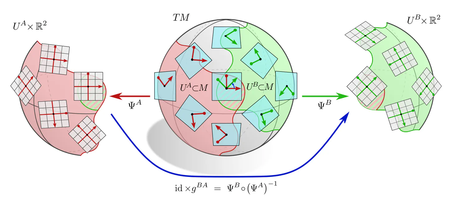
Such a local description becomes necessary when describing CNNs on topologically non-trivial manifolds like the sphere. The implications are similar to those in this post, however, now applying locally:

• Individual feature vectors need to be covariant, which requires that they are associated with a group representation $\rho$ of the covariance group $G$  (in this context called "structure group").
• Network layers need to be covariant as well, here in the sense that the local neural connectivity, e.g. a kernel or bias, needs to be expressible relative to different local reference frames.
• The application of a given local numerical operation is only then independent from the chosen gauge when it is locally gauge equivariant. This requires e.g. $G$-steerable kernels.

The next blog post investigates such coordinate independent CNNs on manifolds in greater detail.

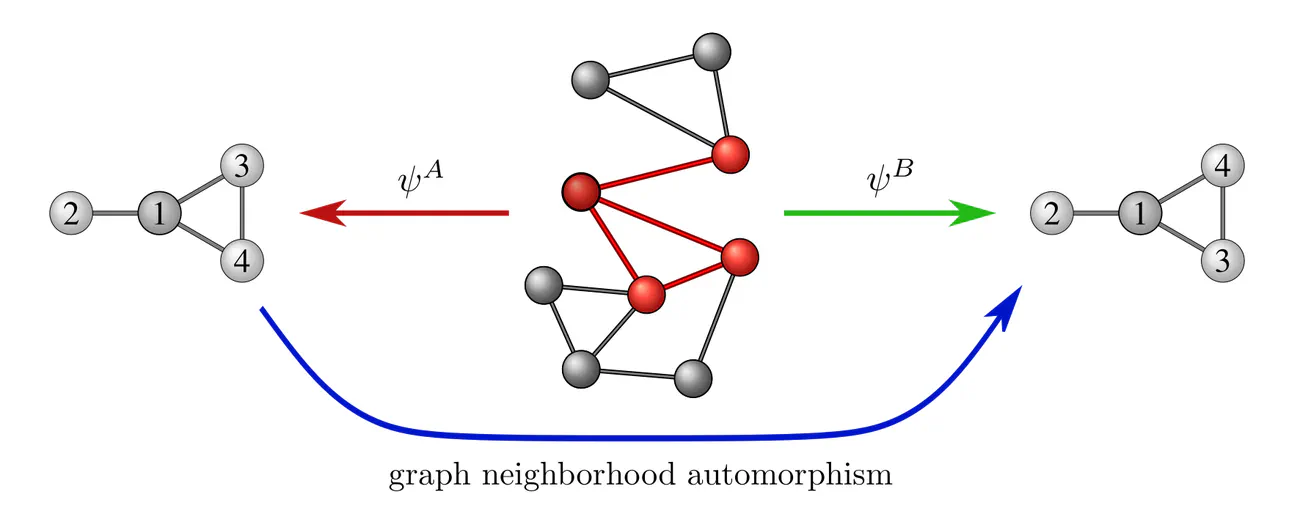
Another example are local graph neighborhood gauges, which assign an independent subgraph labeling to each node neighborhood. Demanding the gauge independence of a local message passing operation requires it to be equivariant under the automorphisms of these graph neighborhoods. Using a slightly different formulation, such "natural graph networks" are described in (de Haan et al., 2020).