Coordinate independent CNNs on Riemannian manifolds
An introduction to equivariant & coordinate independent CNNs – Part 5
This is the last post in my series on equivariant deep learning and coordinate independent CNNs.
- Part 1: Equivariant neural networks – what, why and how ?
- Part 2: Convolutional networks & translation equivariance
- Part 3: Equivariant CNNs & G-steerable kernels
- Part 4: Data gauging, co variance and equi variance
- Part 5: Coordinate independent CNNs on Riemannian manifolds
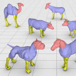
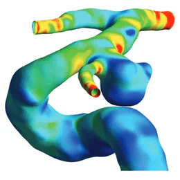
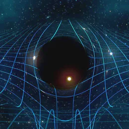
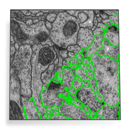
In this post we investigate how convolutional networks are generalized to the differential geometric setting, that is, to process feature fields on manifolds (curved spaces). There are numerous applications of such networks, for instance, to classify, segment or deform meshes, or to predict physical quantities like the wall shear stress on an artery surface or tensor fields in curved spacetime. A differential geometric formulation establishes furthermore a unified framework for more classical models like spherical and Euclidean CNNs.
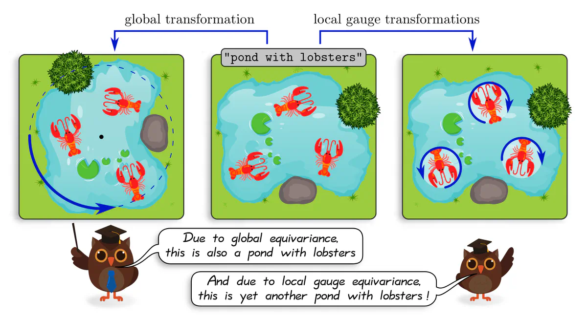
Manifolds do in general not come with a canonical choice of coordinates. CNNs are therefore naturally formulated as a gauge field theory, where the gauge freedom is given by choices of local reference frames, relative to which features and network layers are expressed.
Demanding the coordinate independence (gauge independence) of such CNNs leads inevitably to their equivariance under local gauge transformations. These gauge equivariance requirements correspond exactly to the $G$-steerability constraints from the third post, however, they are here derived in a more general setting.
This post is structured in the following five sections, which cover:
- An intuitive introduction from an engineering viewpoint. It identifies the gauge freedom of choosing reference frames with an ambiguity in aligning convolution kernels on manifolds.
- Coordinate independent feature spaces, which may be represented in arbitrary gauges, and are characterized by their transformation laws when transforming frames.
- The necessity for the gauge equivariance of neural network layers.
- The global isometry equivariance of these operations.
- Applications on different manifolds and with various equivariance properties.
This post’s content is more thoroughly covered in our book Equivariant and Coordinate Independent CNNs, specifically in part II (simplified formulation), part III (fiber bundle formulation), and part IV (applications).
To define CNNs on manifolds, one needs to come up with a reasonable definition of convolution operations. As discussed in the second post of this series, convolutions on Euclidean spaces can be defined as those linear maps that share synapse weights across space, i.e. apply the same kernel at each location.
Kernel alignments as gauge freedom
As it turns out, finding a consistent definition of spatial weight sharing on manifolds is quite tricky. The central issue is the following:
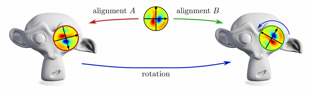
The geometric alignment of convolution kernels on manifolds is inherently ambiguous.
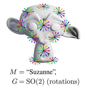
For instance, on the monkey’s head below, it is unclear in which rotation a given kernel should be applied.
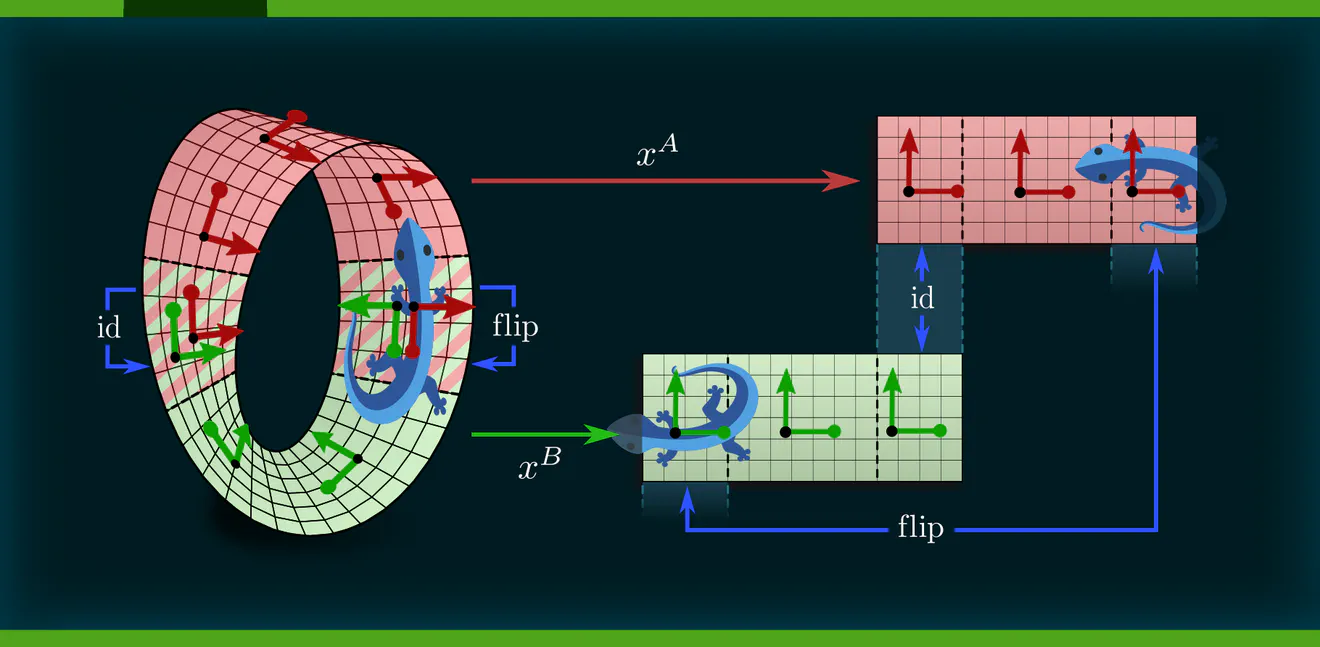
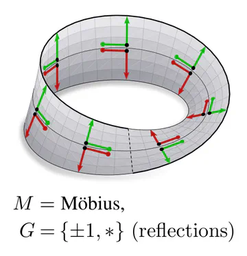
The specific level of ambiguity depends on the manifold’s geometry. For example, the Möbius strip allows for kernels to be aligned along the strip’s circular direction, disambiguating rotations. However, as the strip is twisted, it is a non-orientable manifold, i.e. it does not have a well-defined inside and outside. This implies that the kernel’s reflection remains ambiguous.
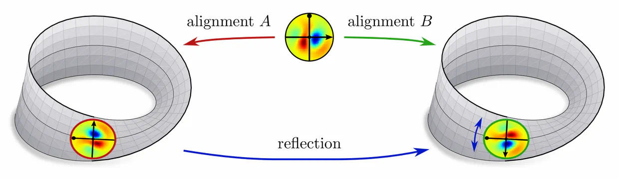
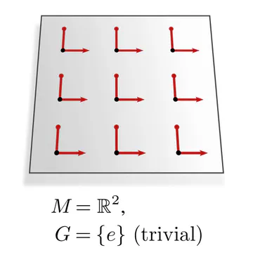
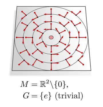
As a third example, consider Euclidean vector spaces $\mathbb{R}^d$. They come canonically with Cartesian coordinates, along which one can uniquely align kernels without any remaining ambiguity. Transformations between “different” alignments are hence trivial, i.e. restricted to the identity map.
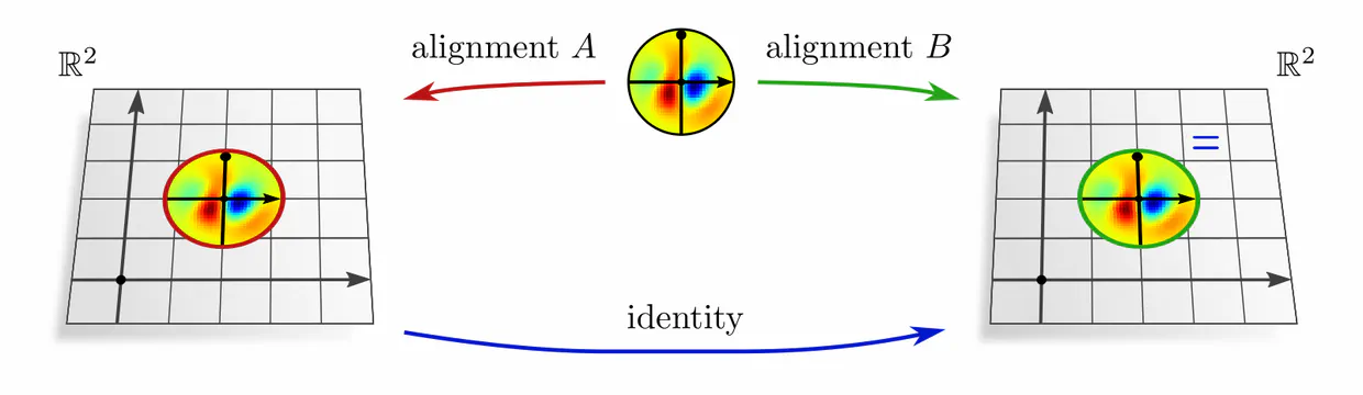
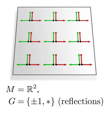
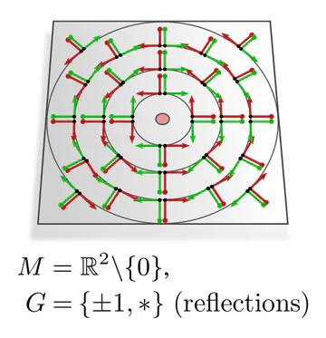
In each of these examples, kernel alignments are specified up to transformations in some matrix group $G\leq \mathrm{GL}(d)$, e.g. rotations $G=\mathrm{SO}(2)$, reflections $G=\{\pm1\}$, or the trivial group $G=\{e\}$. The specific group $G$ depends hereby on the mathematical structure of the manifold. Since we are assuming Riemannian manifolds, we always have access to a metric structure, which allows to align kernels without stretching or shearing them but leaves their rotation and reflection ambiguous, i.e. $G=\mathrm{O}(d)$. That we could reduce $G$ further in the above examples implies that we assumed additional geometric structure, e.g. an orientation (inside/outside) on the monkey head. Any mathematical structure which disambiguates kernel alignments up to transformations in $G$ is called G-structure.
Steerable kernels as gauge independent operations
To remain general, we assume any Riemannian manifolds with any additional $G$-structure for arbitrary $G\leq\mathrm{GL}(d)$. From a practical viewpoint this means that we need to address $G$-ambiguities in kernel alignments when defining convolutions.
Given the context of steerable CNNs from the third post, an obvious solution is to use $G$-steerable kernels. We introduced these kernels there as being $G$-equivariant in the sense that any $G$-transformations of their field of view results in a corresponding $G$-transformations of their response feature vector.
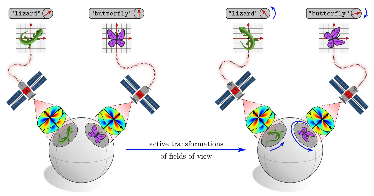
Here we have the slightly different situation of $G$-transformations of the kernels’ alignments, while keeping their fields of view fixed. However, viewed from a kernel’s frame of reference, these two situations are actually indistinguishable! Different alignments of steerable kernels are therefore guaranteed to result in $G$-transformed responses. Such features can hence be viewed as different (covariant) numerical representations of the same abstract feature, just being expressed relative to different frames of reference.
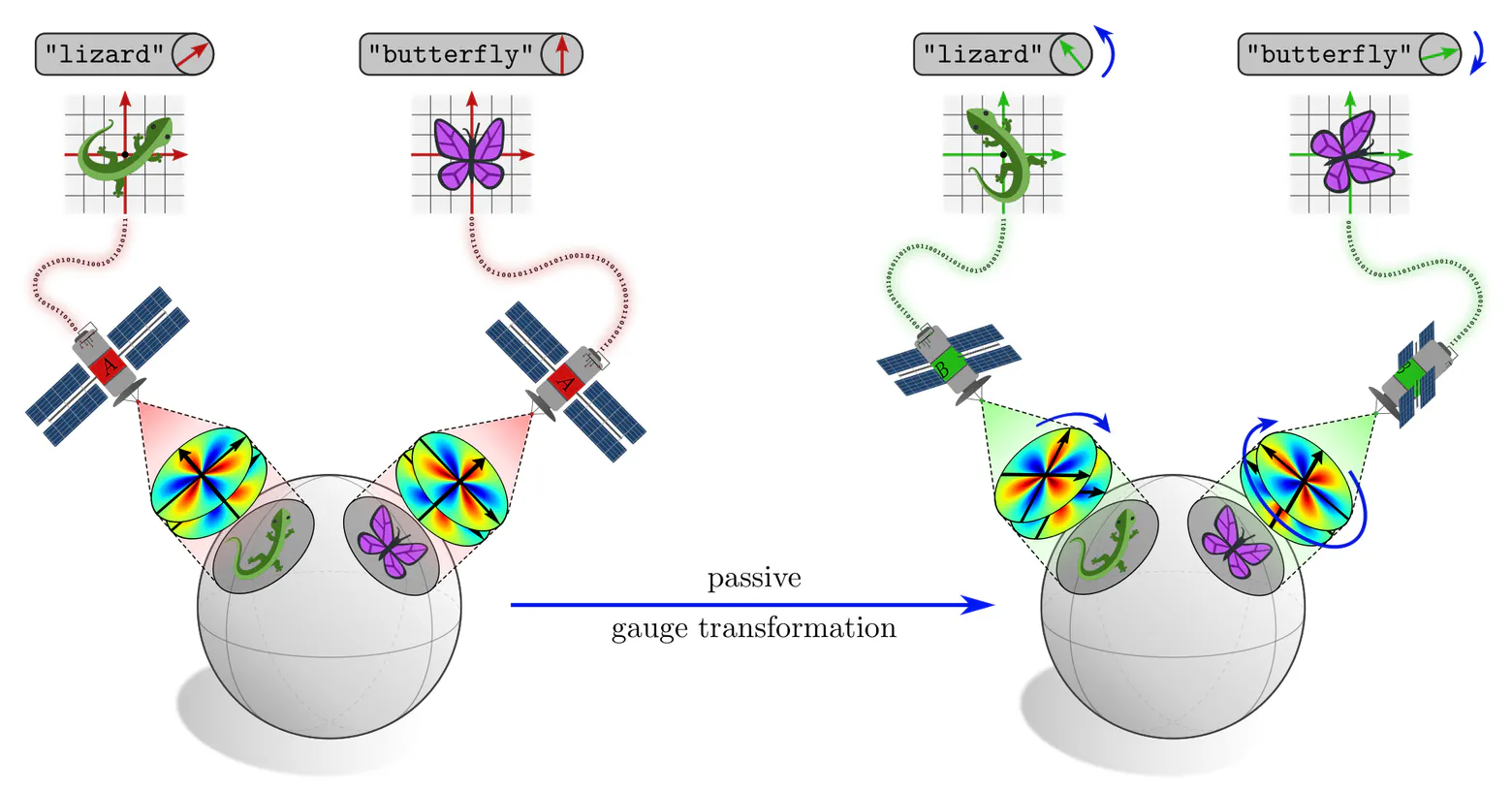
In short, coordinate independent CNNs are just neural networks which apply $G$-steerable kernels, biases or nonlinearities on manifolds with a $G$-structure. The covariance of kernel responses guarantees the independence of the encoded information from particular choices among $G$-ambiguous kernel alignments.
As the visualizations above already suggest, $G$-ambiguities of kernel alignments relate to $G$-ambiguities in choosing reference frames on manifolds.
Any geometric quantities, in particular feature vectors, are required to be $G$-covariant, that is, coordinate independent in the sense that they are expressible relative to any of the ambiguous frames. That convolutional networks need to apply $G$-steerable kernels, biases or nonlinearities follows then by demanding that their layers respect the features’ coordinate independence.
To explain what I mean with “coordinate independent feature spaces”, this section discusses
- tangent spaces and their frames of reference,
- $G$-structures as bundles of geometrically preferred frames, and
- coordinate independent feature vectors.
Tangent vectors and reference frames
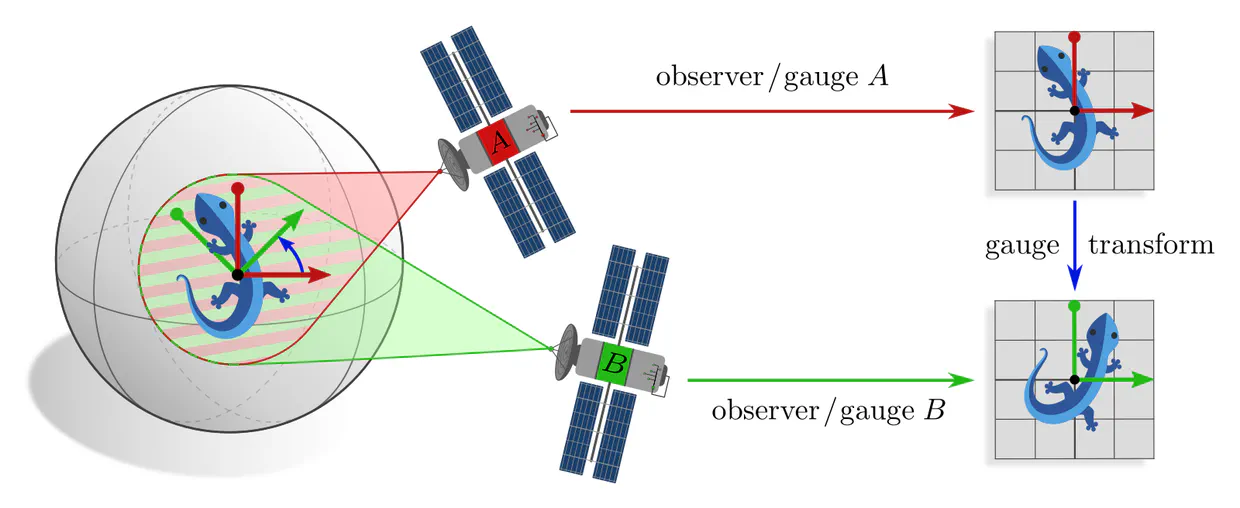
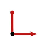
The idea of coordinate independence is best illustrated by the example of tangent vectors. Click on the ❯ arrow to uncover the diagram and the explanatory bullet points step by step.
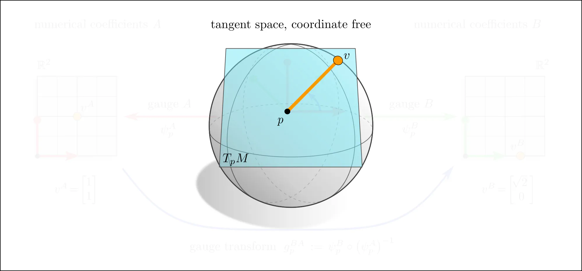
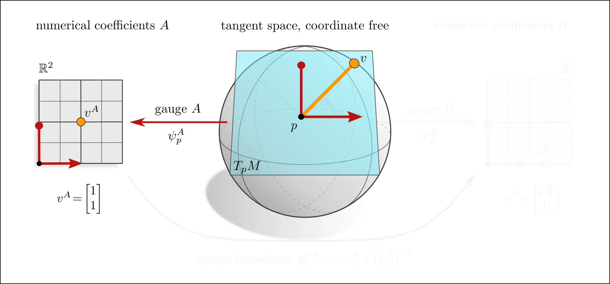
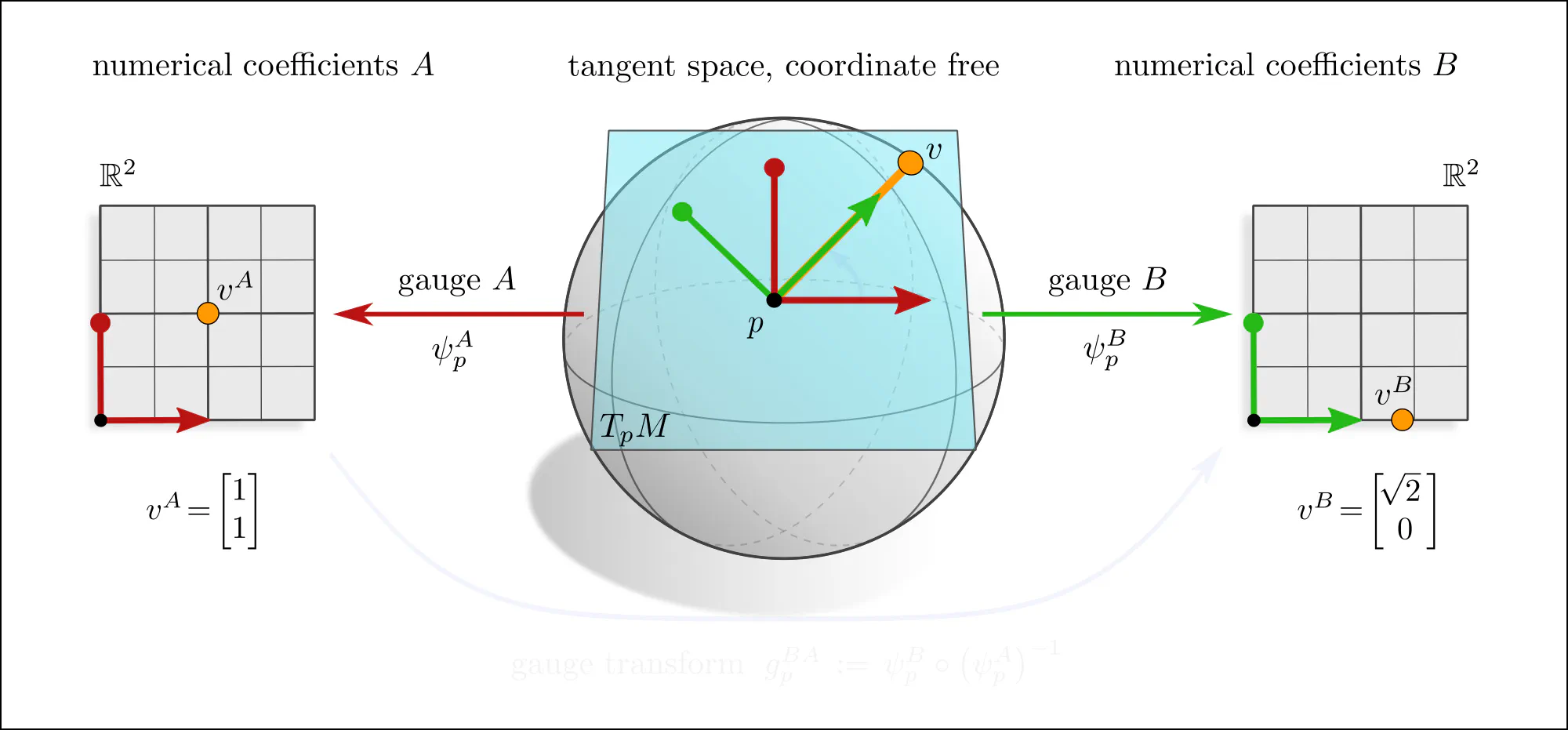
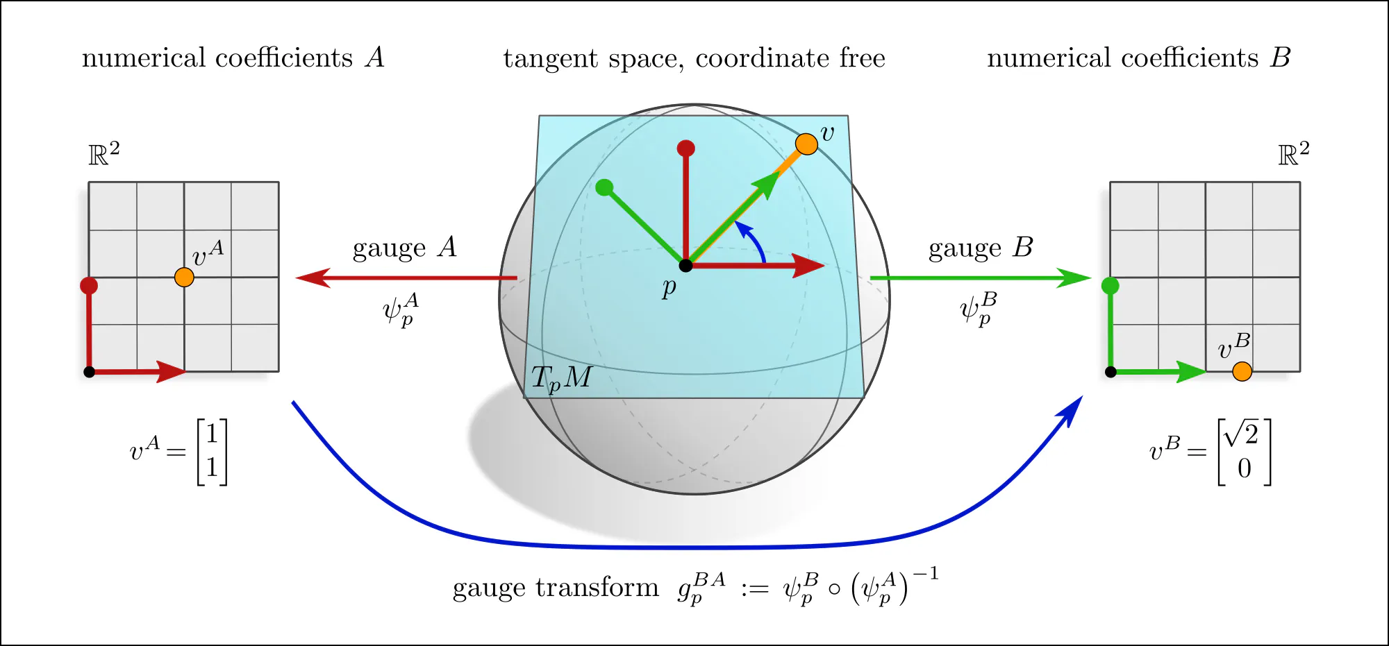
Note how transformations of reference frames and tangent vector coefficients are coupled to each other. This is what is meant when saying that they are associated to each other.
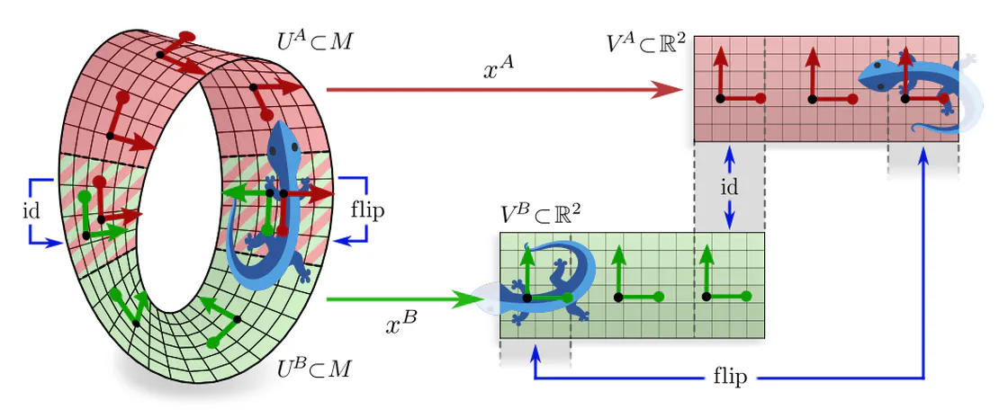
A more formal mathematical description would consider the whole tangent bundle instead of a single tangent space since this allows to capture concepts like the continuity or smoothness of tangent and feature fields. Gauges (local bundle trivializations) correspond then to smooth frame fields (gauge fields) on local neighborhoods $U^A$ or $U^B \subseteq M$ and gauge transformations are defined on overlaps $U^A\cap U^B$ of these neighborhoods.
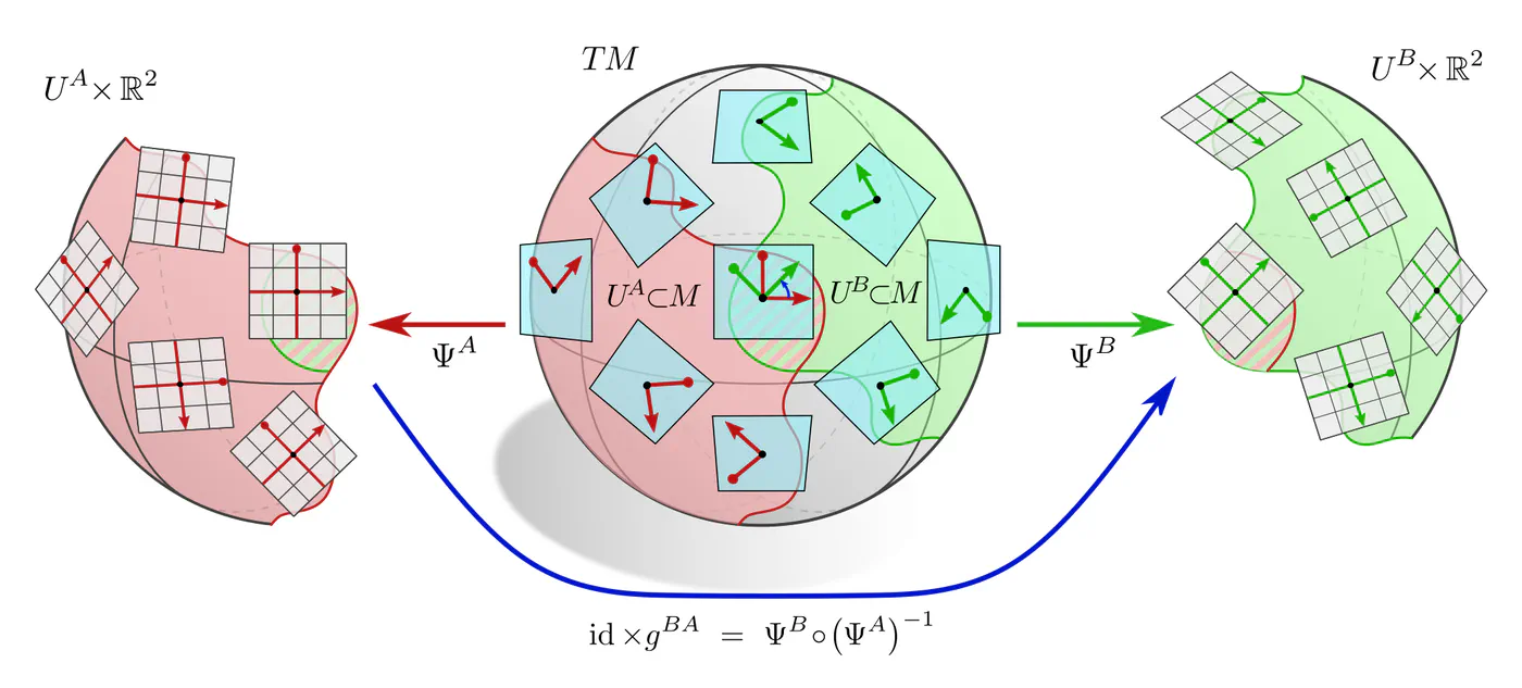
If one picks a coordinate chart $x^A\mkern-3mu: U^A\to V^A\mkern-2mu\subseteq\mkern-1mu\mathbb{R}^d$, frames are induced as coordinate bases with axes $\frac{\partial}{\partial x^A_\mu} \Big|_p$, gauge maps are given by chart differentials $(\psi_p^A)_\mu = dx_\mu^A\big|_p$, and gauge transformations correspond to Jacobians $(g_p^{BA})_{\mu\nu} = \frac{\partial x^B_\mu}{\partial x^A_\nu}$ of chart transition maps. However, the gauge formalism in terms of fiber bundles is more general and more suitable for our purpose.
$G$-structures
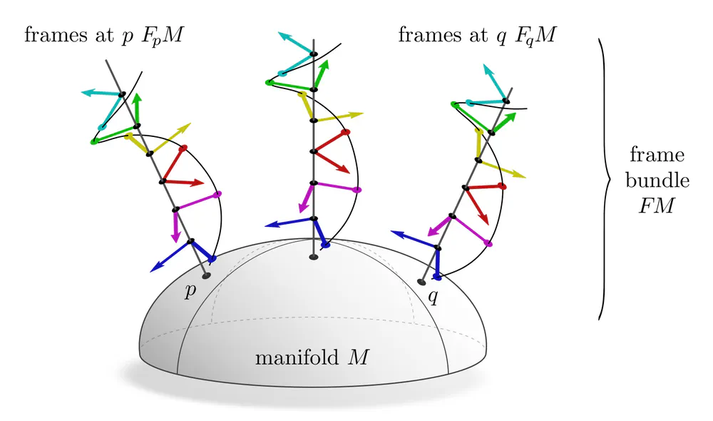
Recall how the manifold’s mathematical structure reduces the ambiguity in kernel alignments such that transformations between them took values in some subgroup $G\leq\mathrm{GL}(d)$. This is made technically precise by $G$-structures, which are $G$-bundles of structurally distinguished frames.
A-priori, a smooth manifold has no additional structure that would prefer any reference frame.
One therefore considers sets $F_pM$ of all possible frames of tangent spaces $T_pM$.
Gauge transformations between such general frames are any invertible linear maps, i.e. take values in the general linear group
Additional structure on smooth manifolds allows to restrict attention to specific subsets of frames. For instance, a Riemannian metric allows to measure distances and angles, and hence to single out orthonormal frames, which are mutually related by rotations and reflections in $G=\mathrm{O}(d)$. Conversely, any $\mathrm{O}(d)$-subbundle of frames determines a unique metric since such sets of orthonormal frames allow for consistent angle and distance measurements. Such equivalences
$G$-structure $\mkern10mu\iff\mkern10mu$ $G$-subbundle of frames
hold for other structure groups $G$ as well. Some more examples:| $\boldsymbol{G}$-structure | $\boldsymbol{G}$-subbundle of frames | structure group $\boldsymbol{G\leq\mathrm{GL}(d)}$ |
|---|---|---|
| smooth structure only | any frames | $\mathrm{GL}(d)$ |
| orientation | right-handed frames | $\mathrm{GL}^+(d)$ |
| volume form | unit-volume frames | $\mathrm{SL}(d)$ |
| Riemannian metric | orthonormal frames | $\mathrm{O}(d)$ |
| pseudo-Riemannian metric | Lorentz frames | $\mathrm{O}(1,\,d\mkern-2mu-\mkern-2mu1)$ |
| metric + orientation | right-handed orthonormal frames | $\mathrm{SO}(d)$ |
| parallelization | frame field (unique frames) | $\{e\}$ |
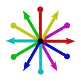
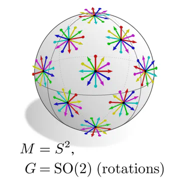
The graphics below give a visual intuition for $G$-structures on different manifolds $M$ and various structure groups $G$. Note that one may have different $G$-structures for the same manifold and group, similar to how one can have different metrics, orientations or volume forms on a manifold.
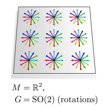
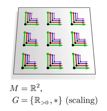
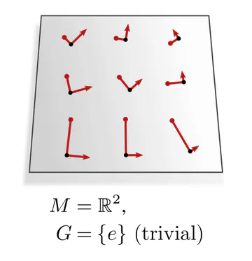
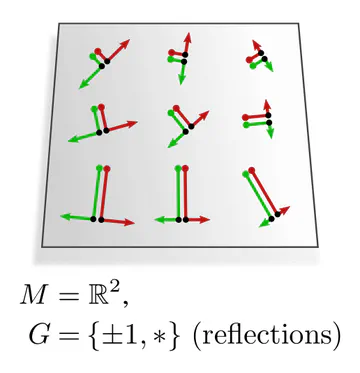
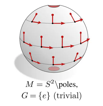
As explained below, each of these $G$-structures implies corresponding convolution operations, whose local gauge equivariance depends on the structure group $G$ and whose global equivariance is determined by the $G$-structure’s global symmetries.
The manifold’s topology may obstruct the existence of a continuous $G$-structure for groups beyond an irreducible structure group. For instance, the Möbius strip is non-orientable, which means that there is no way to disambiguate reflections without introducing a discontinuity. Similarly, the hairy ball theorem implies that frame fields on the sphere ($G=\{e\}$) will inevitably have singularities. This implies:
Any CNN will necessarily have to be $G$-covariant w.r.t. the manifolds irreducible structure group $G$ if the continuity of its predictions are desired.
The manifold's topology might therefore make the use of $G$-steerable kernels strictly necessary!Coordinate independent feature vectors
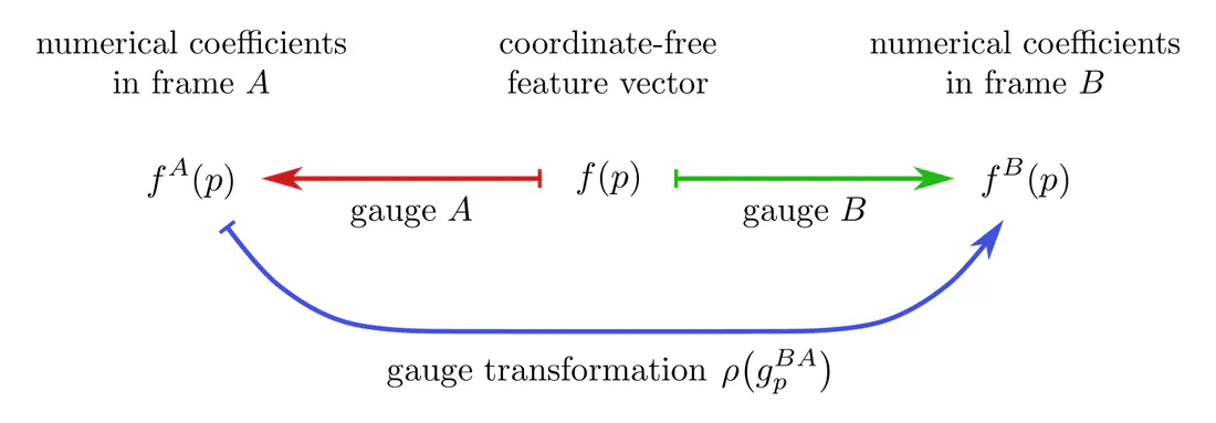
Feature vectors on a manifold with $G$-structure need to be $G$-covariant, i.e. expressible in any frame of the $G$-structure. This requires them to be equipped with a $G$-representation $\rho$, called feature field type, which specifies their gauge transformations when transitioning between frames. Specifically, when $f(p)$ is an abstract $c$-dimensional feature at $p$, it is represented numerically by coefficient vectors $f^A(p)$ or $f^B(p)$ in $\mathbb{R}^c$, which are related by $$f^B(p) \,=\, \rho\big(g_p^{BA}\big) f^A(p)$$ when changing from frame $A$ to frame $B$ via $g_p^{BA}\in G$. Feature vector gauges and gauge transformations between them are again concisely represented via a commutative diagram. Note the similarity to the gauge diagram for tangent vectors above!
This construction allows to model scalar, vector, tensor, or more general feature fields:
| feature field | field type $\boldsymbol{\rho}$ |
|---|---|
| scalar field | trivial representation $\rho(g)=1$ |
| vector field | standard representation $\rho(g)=g$ |
| tensor field | tensor representation $\rho(g) = (g^{-\top})^{\otimes s} \otimes g^{\otimes r}$ |
| irrep field | irreducible representation |
| regular feature field | regular representation |
For a geometric interpretation and specific examples of feature field types, have a look at the examples given in the third post on Euclidean steerable CNNs. In fact, the feature fields introduced here are the differential geometric generalization of the fields discussed there.
Overall, we have the following $G$-associated gauge transformations of objects on the manifold:
- frames transform according to a right action of $(g_p^{BA})^{-1}$
- tangent vector coefficients get left-multiplied by $g_p^{BA}$
- feature vector coefficients transform according to $\rho(g_p^{BA})$
Furthermore, these objects have by construction compatible parallel transporters and isometry pushforwards (global group actions).
Coordinate independent CNNs are built from layers that are 1) coordinate independent and 2) share synapse weights between spatial locations (synapse weights referring e.g. to kernels, biases or nonlinearities). Together, these two requirements enforce the shared weight’s steerability, that is, their equivariance under $G$-valued gauge transformations: $$ \begin{array}{c} \textup{coordinate independence} \\[2pt] \textup{spatial weight sharing} \end{array} \mkern24mu\bigg]\mkern-11mu\Longrightarrow\mkern16mu \textup{$G$-steerability / gauge equivariance} $$
Kernels in geodesic normal coordinates
In contrast to Euclidean spaces, the local geometry of a Riemannian manifold might vary from point to point. It is therefore not immediately clear how convolution kernels should be defined on it and how they could be shared between different locations. A common solution is to define kernels as usual on flat Euclidean space and to apply them on tangent spaces instead of the manifold itself.
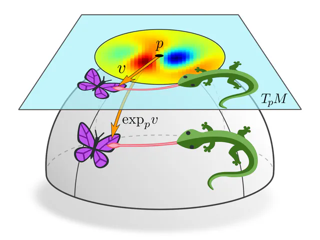
To match the kernel with feature fields it needs to be projected to the manifold, for which we leverage the Riemannian exponential map. Equivalently, one can think about this as pulling back the feature field from the manifold to the tangent spaces. When being expressed in a gauge, this corresponds to applying the kernel in geodesic normal coordinates.
Gauge equivariance
The equivariance requirement on kernels follows by the same logic as discussed in the previous post: a-priori, $G$-covariance just requires consistent gauge transformation laws of kernels, but weight sharing can only remain coordinate independent when kernels are constrained to be $G$-steerable.
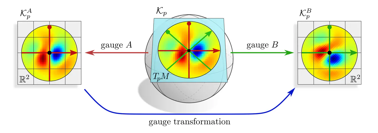
G-covariance : Assume that we are given a coordinate free kernel $\mathcal{K}_p$ on a tangent space $T_pM$. It can of course be expressed in different frames of reference. The coordinate expressions $\mathcal{K}_p^A$ and $\mathcal{K}_p^B$, defined on $\mathbb{R}^d$, are then related by some gauge transformation law which is derived here.
G-equivariance : In the case of convolutions, there is no initial kernel $\mathcal{K}_p$ on $T_pM$ given, but rather a kernel $K$ on $\mathbb{R}^d$ which should be shared over all tangent spaces. Choosing kernel alignments $A$ or $B$ corresponds mathematically to defining $\mathcal{K}_p$ by setting $\mathcal{K}_p^A=K$ or $\mathcal{K}_p^B=K$. However, the choice of gauge/frame/alignment is ambiguous, and one will in general obtain incompatible results.
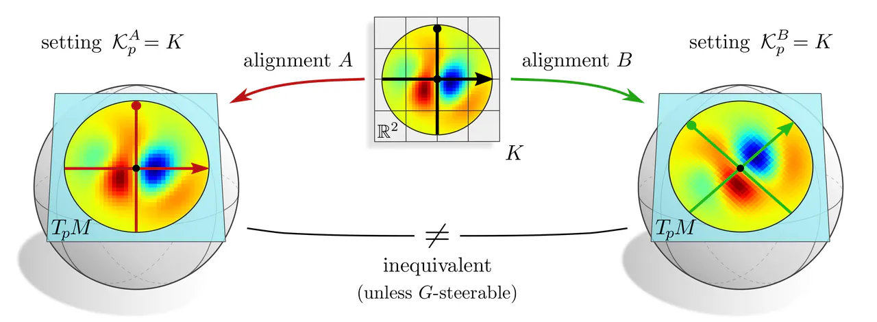
Aligning $K$ in any single gauge would prefer that specific gauge, and therefore break coordinate independence. The solution is to treat all gauges equivalently, that is to set $$ \mathcal{K}_p^X = K \mkern24mu\textup{for }\textit{any }\textup{gauge $X$ of the $G$-structure,} $$ which can be interpreted as an additional weight sharing over all frames of the $G$-structure. Doing so turns the covariance conditions of the form $$ \mathcal{K}_p^B\ =\ g_p^{BA} \circ \mathcal{K}_p^A \circ \big( g_p^{BA} \big)^{-1} $$ for any gauges $A$ and $B$ into $G$-equivariance constraints $$ K\ =\ g \circ K \circ g^{-1} \qquad\forall\ g\in G. \mkern-43mu $$ These are exactly the $G$-steerability constraints known from steerable CNNs on Euclidean spaces.
Example : To get an intuition for the role of steerable kernels, let's consider the example of a reflection group structure. As discussed in the third post, two possible field types $\rho$ for the reflection group are the trivial and the sign-flip representation. They correspond to scalar and pseudoscalar fields, whose numerical coefficients stay invariant and negate under frame reflections, respectively. Reflection-steerable kernels that map from scalar to pseudoscalar fields were constrained to be antisymmetric.
Applying such an antisymmetric kernel in some gauge $A$ to a scalar field results in some response field in gauge $A$. If the kernel is instead applied in the reflected gauge $B$, the response field will due to the kernel's antisymmetry end up negated. This transformation behavior does indeed identify the response field as being of pseudoscalar type.
You can check equivalent properties for any of the other pairs of field types and their steerable kernels from the third post. The difference here is that we are considering passive transformations of frames and kernel alignments instead of active transformations of signals. As only the relative alignment of kernels and signals matters, the behavior is ultimately equivalent.
Similar $G$-steerability requirements as for convolution kernels can be derived for ${1\mkern-6.5mu\times\mkern-5.5mu1}$-convolutions, bias vectors and nonlinearities.
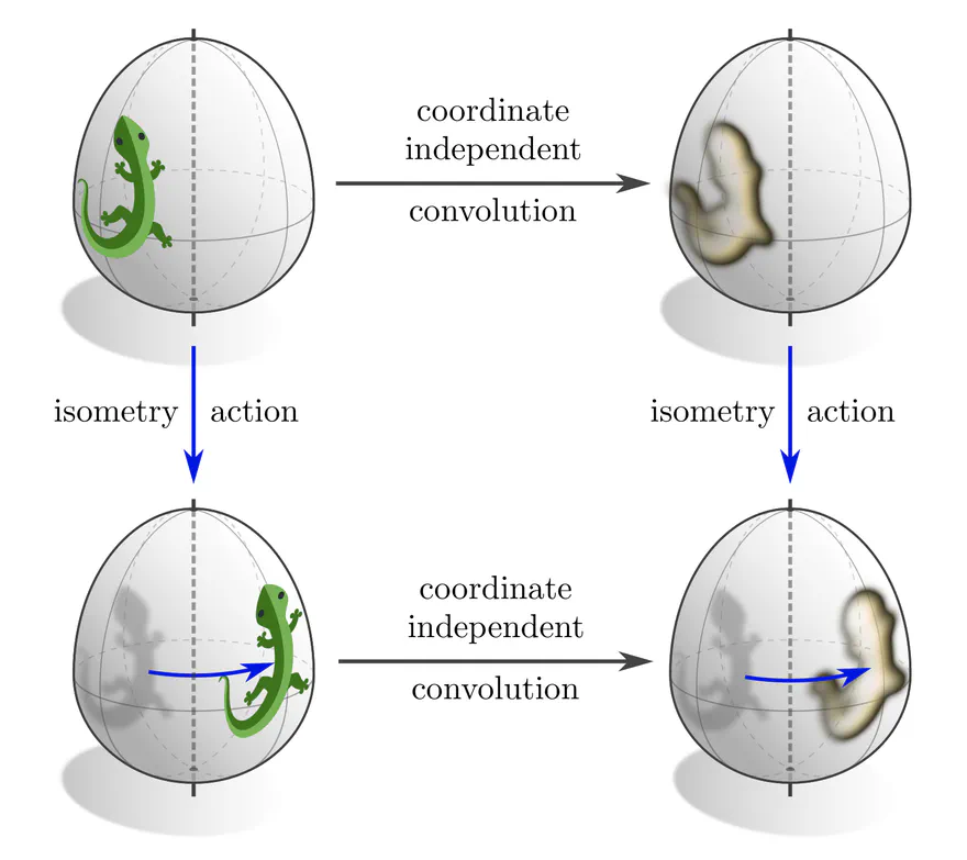
Classically, convolutional networks are those networks that are equivariant w.r.t. symmetries of the space they are operating on. For instance, conventional CNNs on Euclidean spaces commute with translations, Euclidean steerable CNNs commute with affine groups, and spherical CNNs commute with $\mathrm{SO}(3)$ rotations. Similarly, one may ask in how far coordinate independent CNNs are equivariant w.r.t. isometries, which are the symmetries of Riemannian manifolds (distance preserving diffeomorphisms).
The following section investigates the prerequisites for a layer’s isometry equivariance prior to convolutional weight sharing. In the one thereafter we apply the results to coordinate independent convolutions.
Isometry invariant kernel fields
Our main theorem regarding the isometry equivariance of coordinate independent CNNs establishes the mutual implication
isometry equivariant layer $\mkern10mu\iff\mkern10mu$ isometry invariant neural connectivity ,
which applies either to the manifold's full isometry group $\mathrm{Isom}(M)$ or to any of its subgroups. For linear layers this requires- weight sharing of kernels across isometry orbits (points related by the isometry action) and
- the kernels' steerability w.r.t. their respective stabilizer subgroup.
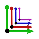
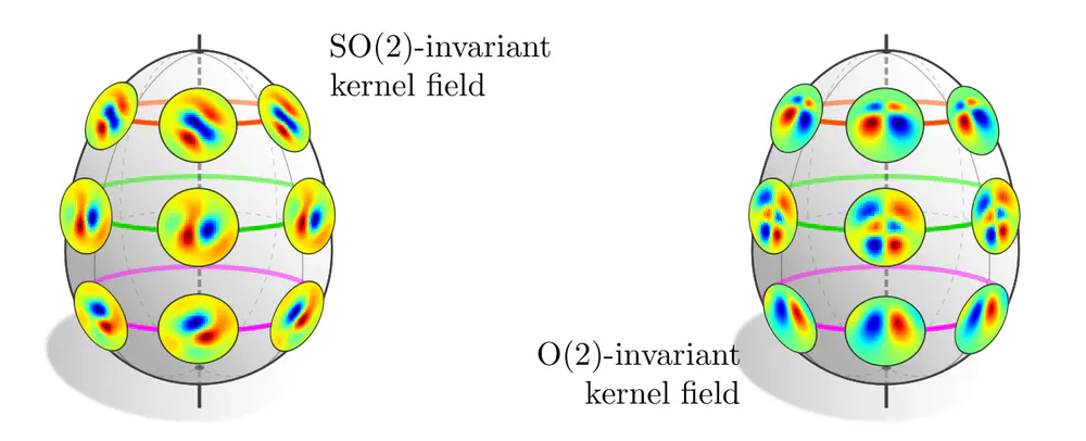
Two examples are shown below. The first one considers the rotational isometries of an egg-shaped manifold, whose orbits are rings at different heights and the north and south pole. In principle, equivariance does not require weight sharing across the whole manifold, but just on the rings, allowing for different kernels on different rings. The stabilizer subgroups on the rings are trivial, leaving the kernels themselves unconstrained. The second example considers an $\mathrm{O}(2)$-invariant kernel field. While the orbits remain the same, their stabilizer subgroups are extended by reflections, such that the kernels are required to become reflection-steerable. The specific steerability constraints depend of course on the field types between which the kernels are supposed to map.
A special case are manifolds like Euclidean spaces or the sphere $S^2$ – they are homogeneous spaces, which means that their isometry group acts transitively, i.e. allows to map any point $p$ to any other point $q$. Consequently, there exists only one single orbit and kernel. Another one of our theorems asserts:
Isometry equivariant linear layers on homogeneous spaces are necessarily convolutions.
Isometry equivariance of convolutions
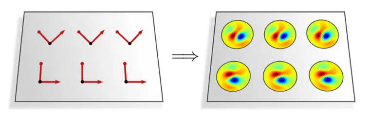
Coordinate independent convolutions rely on specific convolutional kernel fields, constructed by sharing a single $G$-steerable kernel along the frames of a $G$-structure. The convolutions’ isometry equivariance depends consequently on the extent of invariance of these kernel fields.
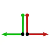
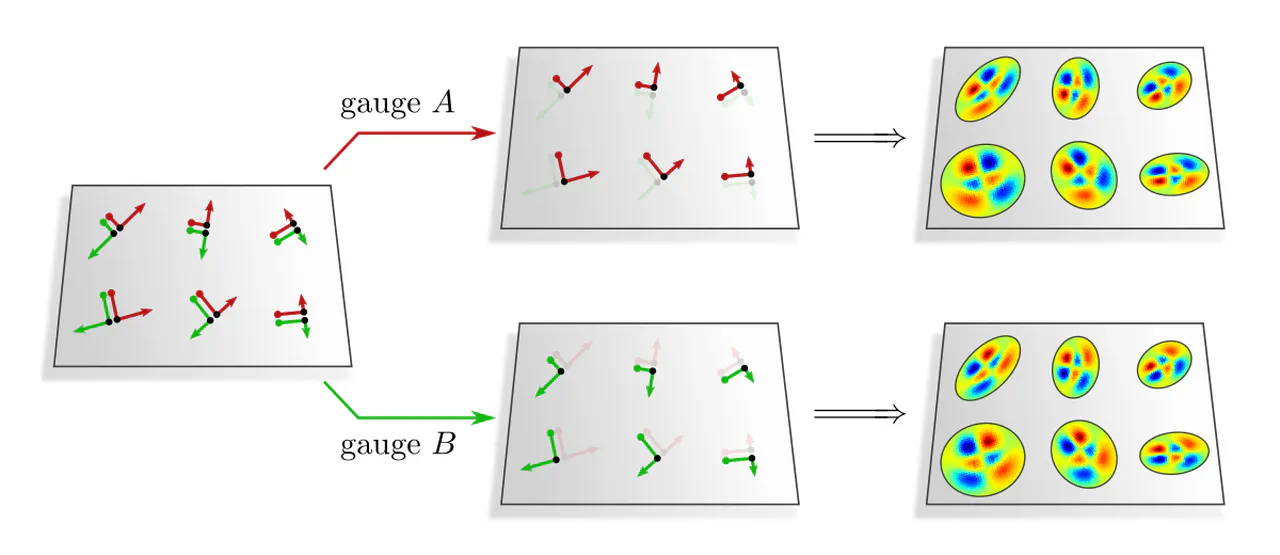
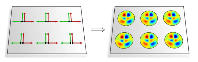
As a first example, consider the $\{e\}$-structure (frame field) in the left figure below. Its invariance under horizontal translations leads to an equivalent symmetry in kernel fields – the corresponding convolutions are therefore equivariant under horizontal translations. The translation and reflection invariance of the reflection-structure in the right figure is similarly carried over to its kernel fields, thus implying translation and reflection equivariant convolutions.
The observation that convolutional kernel fields inherit the symmetries of their underlying $G$-structure holds in general. Based on this insight, we have the following theorem:
Coordinate independent CNNs are equivariant w.r.t. those isometries that are symmetries of the $G$-structure.
This allows us to design equivariant convolutions on manifolds by designing $G$-structures with the appropriate symmetries! More examples of $G$-structures and the implied equivariance properties are discussed in the applications section below.
Diffeomorphism and affine group equivariance
Beyond isometries, one could consider general diffeomorphisms. Any operation that acts pointwise, for instance bias summation or ${1\mkern-6.5mu\times\mkern-5.5mu1}$-convolutions, can indeed be made fully diffeomorphism equivariant by choosing $G=\mathrm{GL}(d)$. However, that does not apply to convolutions with spatially extended kernels as their projection to the manifold via the exponential map depends on the metric structure and does therefore only commute with isometries, i.e. metric preserving diffeomorphisms. To achieve diffeomorphism equivariance, steerable kernels would have to be replaced by steerable partial differential operators.
Specifically on Euclidean spaces, the Riemannian exponential map does not only commute with isometries in the Euclidean group $\mathrm{E}(d) =$ $(\mathbb{R}^d,+)\rtimes \mathrm{O}(d)$, but also with more general affine groups $\mathrm{Aff}(G)$ $=$ $(\mathbb{R}^d,+)\rtimes G$ for arbitrary $G\leq\mathrm{GL}(d)$. Choosing $\mathrm{Aff}(G)$-invariant $G$-structures on Euclidean spaces leads therefore to $\mathrm{Aff}(G)$-equivariant convolutions which turn out to be exactly the Euclidean steerable CNNs from the third post.
Our gauge theoretic formulation of feature vector fields and network layers is quite general: we were able to identify more than 100 models from the literature as specific instantiations of coordinate independent CNNs. While the authors did not formulate their models in terms of $G$-structures and field types $\rho$, these geometric properties follow from the weight sharing patterns and kernel symmetries that they proposed.
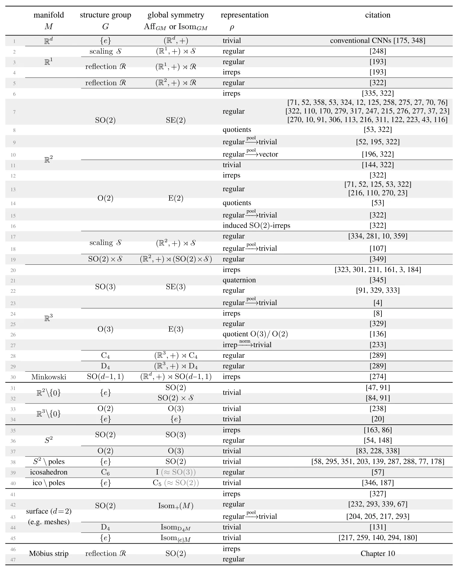
The next sections give a brief overview of the different model categories in this literature review. As the networks’ local and global equivariance properties correspond to symmetries of the underlying $G$-structures, they are intuitively visualized by plots of the latter.
Euclidean steerable CNNs
All of the models in the first 30 lines are steerable CNNs on Euclidean spaces, that is, conventional convolutions with $G$-steerable kernels. From the differential geometric viewpoint, they correspond to $G$-structures that are $\mathrm{Aff}(G)$-invariant, i.e. invariant under translations and $G$-transformations. This affine symmetry of the $G$-structures implies the convolutions’ $\mathrm{Aff}(G)$-equivariance. Aside from the choice of structure group, these models differ mainly in the feature fields types $\rho$ that they operate on.
The major new insight in comparison to the classical formulation of equivariant CNNs is that coordinate independent CNNs do not only describe the models’ global $\mathrm{Aff}(G)$-equivariance, but also their local gauge equivariance, i.e. generalization over local $G$-transformations of patterns.
For more details on Euclidean steerable CNNs, have a look at the third post of this series.
Polar and hyperspherical convolutions on Euclidean spaces
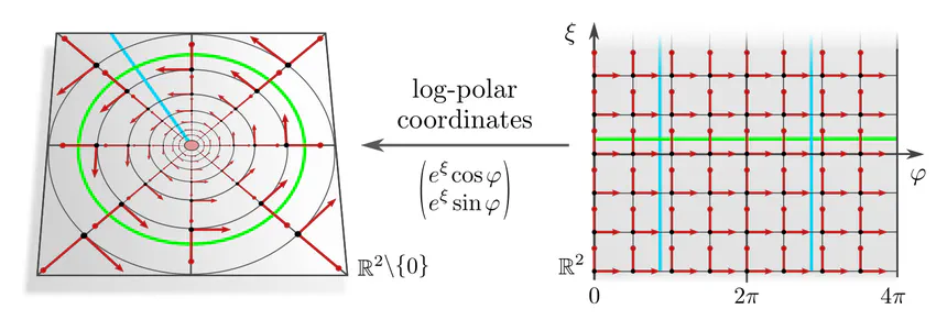
Instead of using polar coordinates with an isometric radial part one may use log-polar coordinates (line 32), whose frames scale exponentially with the radius. This $\{e\}$-structure is not only rotation invariant but also invariant under rescaling of $\mathbb{R}^2\backslash\{0\}$ and implies hence rotation and scale equivariant convolutions (Esteves et al., 2018). It is easily implemented as a conventional Euclidean convolution after resampling the feature field in the coordinate chart (pulling it from the left to the right side of the figure). Rotations and scaling correspond in the chart to horizontal and vertical translations, respectively.
Higher-dimensional analogs of these architectures on $\mathbb{R}^d\backslash\{0\}$ rely on convolutions on $d\mkern-3mu-\mkern-4.5mu1$-dimensional spherical shells at different radii (lines 33,34); see here for more infos and visualizations.
Spherical CNNs
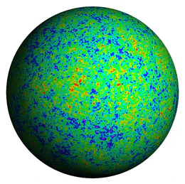
Spherical CNNs are relevant for processing omnidirectional images from 360° cameras, the cosmic microwave background, or climate patterns on the earth’s surface. They come in two main flavors:
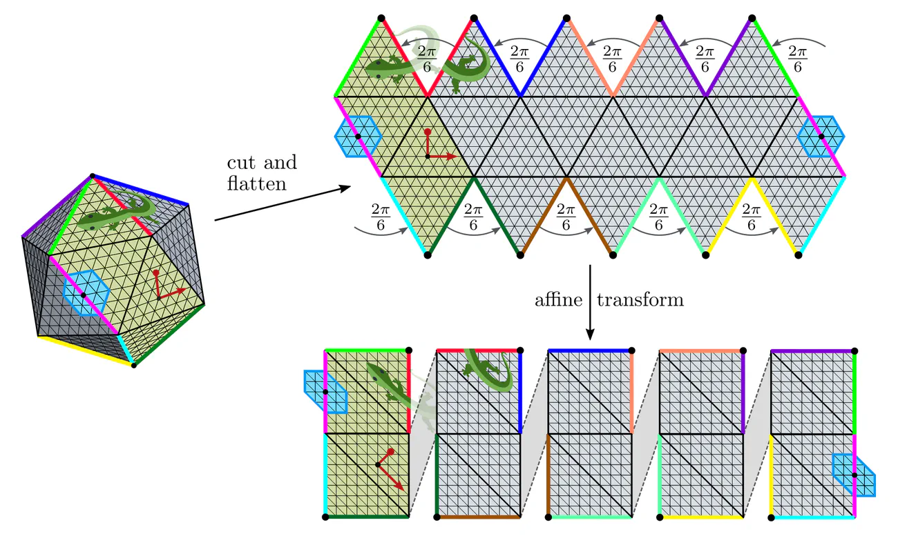
The spherical geometry may furthermore be approximated by that of an icosahedron (lines 39,40). An advantage of this approach is that the icosahedron is locally flat and allows for an efficient implementation via Euclidean convolutions on the five visualized charts. The non-trivial topology and geometry manifests in parallel feature transporters along the cut edges (colored chart borders). Icosahedral CNNs appear again in the two flavors above, where $\mathrm{SO}(2)$ is typically approximated by the cyclic group $\mathrm{C}_6$, which is a symmetry of the utilized hexagonal lattice.
Möbius CNNs
Assuming the strip to be flat (have zero curvature), such convolutions are conveniently implemented in isometric coordinate charts. When splitting the strip in two charts as shown below, their transition map will at one end be trivial and at the other be related by a reflection. In an implementation, one can glue the two chart codomains at their trivial transition ($\mathrm{id}$). The only difference to reflection-steerable convolutions on Euclidean space is that the strip needs to be glued at the non-trivial cut ($\mathrm{flip}$). This is implemented via a parallel transport padding operation which pads both ends of the strip with spatially reflected and gauge reflected features from the respective other end.
If you are interested in learning more about Möbius convolutions, check out our implementation on github and the explanations and derivations in chapter 10 of our book.
General surfaces
An alternative approach is to address the ambiguity of kernel alignments on surfaces by computing them via some sort of heuristic. The examples in line 45 of the table above do this by aligning kernels along principal curvature directions of their embedding in $\mathbb{R}^3$ or along the embedding space’s z-axis, by parallel transporting kernels, via a local PCA of nodes, or by convolving over texture maps. In the framework of coordinate independent CNNs, these heuristics are interpreted as specifying $\{e\}$-structures on the manifold. Note that the heuristics may be instable under deformations, may not everywhere be well defined, and are likely to have singularities - the latter is actually unavoidable on non-parallelizable surfaces!
The main points discussed in this post are:
- The geometric alignment of convolution kernels on a manifolds is often inherently ambiguous. This ambiguity can be identified with the gauge freedom of choosing reference frames.
- The specific level of ambiguity depends on the manifold's mathematical structure. $G$-structures disambiguate frames up to $G$-valued gauge transformations.
- Feature vectors and other mathematical objects on the manifold should be $G$-covariant, i.e. expressible relative to any frame from the $G$-structure (coordinate independent). They transform according to a $G$-representation $\rho$, called field type. Gauge transformations of frames, tangent and feature vector coefficients are synchronized, that is, their fiber bundles are $G$-associated.
- In order for the spatial weight sharing of a kernel to remain coordinate independent, the kernel is required to be $G$-steerable, i.e. equivariant under gauge transformations. The same holds for other shared operations like bias summation or nonlinearities.
- A layer is isometry equivariant iff its neural connectivity is invariant under isometry actions.
- For convolutions, this neural connectivity is given by a kernel field whose symmetries coincide by construction with those of the $G$-structure. Convolutions are therefore equivariant under those isometries that are symmetries of the $G$-structure.
While being somewhat abstract, our differential geometric formulation of coordinate independent CNNs in terms of fiber bundles is highly flexible and allows to unify a wide range of related work in a common framework. It even includes completely non-equivariant models like those in line 45 of the table above – they correspond in our framework to asymmetric $\{e\}$-structures.
Of course there are neural networks for processing feature fields that are not explained by our formulation of coordinate independent CNNs. Such models could, for instance, rely on spectral operations, involve multi-linear correlators of feature vectors, operate on renderings, be based on graph neural networks, or on stochastic PDEs like diffusion processes, to name but a few alternatives. Importantly, these approaches are compatible with our definition of feature spaces in terms of associated $G$-bundles, they are just processing these features in a different way.
An interesting extension would be to formulate a differential version of coordinate independent CNNs, replacing our spatially extended steerable kernels by steerable partial differential operators. As mentioned above, this would allow for diffeomorphism equivariant CNNs.
Lastly, I would like to mention gauge equivariant neural networks for lattice gauge theories in fundamental physics, for instance (Boyda et al., 2021) or (Katsman et al., 2021). The main difference to our work is that their gauge transformations operate in an “internal” quantum space instead of spatial dimensions. However, both are naturally formulated in terms of associated fiber bundles. Their models are furthermore spatially equivariant and are in this sense compatible with our gauge equivariant CNNs.
Maurice Weiler
Deep Learning Researcher
I’m a researcher working on geometric and equivariant deep learning.
Image references
- Lizards and butterflies adapted under the Creative Commons Attribution 4.0 International license by courtesy of Twitter.
- Mesh segmentation rendering from Sidi et al. (2021).
- Artery wall stress rendering from Shiba et al. (2017).
- Spacetime visualization from WGBH.
- Cosmic microwave background adapted from Tegmark et al. (2023).
- Electron microscopy of neural tissue adapted from the ISBI 2012 EM segmentation challenge.
- Lobsters adapted under the Apache license 2.0 by courtesy of Google.
- Owl teacher adapted from Freepik